Lecture 7 - Case Studies

Overview

In this lecture, we cover some key aspects of being a data scientist and some principles for exploratory data analysis.

We also cover two case studies:

NYC airbnb
food prices for nutrition

References

R for Data Science (2e) (Wickham et al. 2023)

What makes a good data scientist?

From Jeff Goldsmith (Columbia):

You need data skills
- data wrangling
- reproducibility
- communication
- analytics and modeling
You also need a mindset:
- intellectual curiosity
- ability to solve problems
- interest in domain area

Problem solving

Quote from Chris Volinsky, “How Industry Views Data Science Education in Statistics Departments”

I’ve interviewed a lot of people over the years… recently, when people have an interview, I ask a single question that I think tries to get at the point of problem solving. The question I ask is along the lines of:

“Imagine you had access to a database of 100 million mobile devices. What questions would you ask? What types of things do you think you could learn, and how would you go about doing it?”

Exploratory Data Analysis

From R for Data Science (2e):

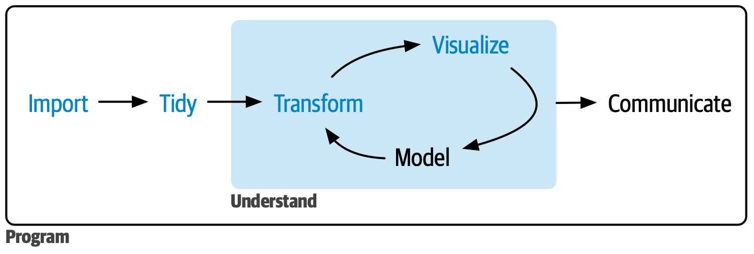
Exploratory data analysis (EDA) is an iterative cycle:

Generate questions about your data.
Search for answers by visualizing, transforming, and modelling your data.
Use what you learn to refine your questions and/or generate new questions.

Often, insightful questions will only become clear after some exploration of the data.

Two helpful questions to start with are:

What type of variation occurs within my variables?

Variation is the tendency of the values of a variable to change from measurement to measurement.
What type of covariation occurs between my variables?

Covariation is the tendency for the values of two or more variables to vary together in a related way.

Case Study: New York City Airbnb Data

This following notebook is an annotated Python script translation of Jeff Goldsmith’s course P8105: Data Science I at the Biostatistics Department at the Columbia School of Public Health.

Data source

Our data was accessed, according to the P8105 site, from Inside Airbnb on September 2, 2017. Inside Airbnb provides some visualizations of the NYC Airbnb data here, where you can see maps showing type of room, activity, availability, and listings per host for all NYC Airbnb listings.

Brainstorm questions for reference

Where are max and min air bnb prices?
- what are average prices?
- What factors affect prices?
Where are prices going up and down over time?
What’s the relationship between number of reviews and average review?
Does room type affect availability?
What’s the location of the unit?
- What areas are popular?
- Popularity = number of units? Average price?
Are there repeat hosts?
- If so, what does that mean?

Let’s start coding!

import pandas as pd
import numpy as np
import matplotlib.pyplot as plt
import seaborn as sns
import plotly.express as px

## Set palette for categorical display
sns.set_palette('Set2')
sns.color_palette("Set2")

Reading the data

The file nyc_airbnb contains a single dataframe nyc_airbnb with 40,753 rows of data on 17 variables.

id: listing id
review_scores_location: 0-5 stars converted into a 0-10 scale
name: listing name
host_id: host id
host_name: host name
neighbourhood_group: NYC borough
neighbourhood: NYC neighborhood
latitude: listing latitude
longitude: listing longitude
room_type: type of listing (Entire home/apt, Private room, Shared room)
price: listing price
minimum_nights: required minimum nights stay
number_of_reviews: total number of reviews
last_review: date of last review
reviews per month: average number of reviews per month
calculated_host_listings_count: total number of listings for this host
availability_365: number of days listing is available out of 365

nyc_airbnb = pd.read_csv('../data/nyc_airbnb.csv')
nyc_airbnb.head()

	id	review_scores_location	name	host_id	host_name	neighbourhood_group	neighbourhood	long	lat	room_type	price	minimum_nights	number_of_reviews	last_review	reviews_per_month	calculated_host_listings_count	availability_365
0	7949480	10.0	City Island Sanctuary relaxing BR & Bath w Par...	119445	Linda & Didier	Bronx	City Island	-73.788680	40.852054	Private room	99	1	25	4/23/17	1.59	1	170
1	16042478	NaN	WATERFRONT STUDIO APARTMENT	9117975	Collins	Bronx	City Island	-73.788607	40.853491	Private room	200	7	0	NaN	NaN	1	180
2	1886820	NaN	Quaint City Island Community.	9815788	Steve	Bronx	City Island	-73.783052	40.841144	Entire home/apt	300	7	0	NaN	NaN	1	365
3	6627449	10.0	Large 1 BDRM in Great location	13886510	Arlene	Bronx	City Island	-73.786609	40.849775	Entire home/apt	125	3	12	10/24/16	0.54	1	335
4	5557381	10.0	Quaint City Island Home	28811542	Phoebe	Bronx	City Island	-73.789328	40.850024	Private room	69	3	86	4/22/17	3.63	1	352

Summary statistics

Max-min stats for prices

# Compute max, min, and mean of the 'price' column
max_price = nyc_airbnb['price'].max()
min_price = nyc_airbnb['price'].min()
mean_price = nyc_airbnb['price'].mean()

print(f"Max price: {max_price}")
print(f"Min price: {min_price}")
print(f"Mean price: {mean_price}")

Max price: 10000
Min price: 10
Mean price: 145.2863592864329

## Summary stats
nyc_airbnb.describe()

	id	review_scores_location	host_id	long	lat	price	minimum_nights	number_of_reviews	reviews_per_month	calculated_host_listings_count	availability_365
count	4.075300e+04	30716.000000	4.075300e+04	40753.000000	40753.000000	40753.000000	40753.000000	40753.000000	31454.000000	40753.000000	40753.000000
mean	9.912016e+06	9.417991	3.059031e+07	-73.955952	40.730776	145.286359	3.964861	16.409467	1.312114	1.662675	134.081614
std	5.582254e+06	0.836230	3.267980e+07	0.041214	0.053690	209.946665	13.194728	29.973090	1.757380	2.159644	137.809093
min	2.515000e+03	2.000000	7.200000e+01	-74.240843	40.499794	10.000000	1.000000	0.000000	0.010000	1.000000	0.000000
25%	4.995083e+06	9.000000	4.857042e+06	-73.983946	40.692356	70.000000	1.000000	1.000000	0.250000	1.000000	0.000000
50%	1.001931e+07	10.000000	1.805129e+07	-73.957210	40.724119	100.000000	2.000000	4.000000	0.750000	1.000000	84.000000
75%	1.496799e+07	10.000000	4.664988e+07	-73.940474	40.764489	170.000000	3.000000	18.000000	1.910000	2.000000	277.000000
max	1.851999e+07	10.000000	1.284849e+08	-73.711750	40.912164	10000.000000	1250.000000	432.000000	125.920000	35.000000	365.000000

Factors that might affect prices

We first compare the distribution of prices across neighborhood groups:

# Histogram of price grouped by neighbourhood_group
g = sns.FacetGrid(data=nyc_airbnb, col='neighbourhood_group', 
                  col_wrap=5,hue='neighbourhood_group',
                  xlim = (0, 250))
g.map(sns.histplot, 'price',binwidth=3, element='step', common_norm=False)
g.add_legend(title = 'Neighbourhood Group')
g.set_titles('{col_name}')

plt.show()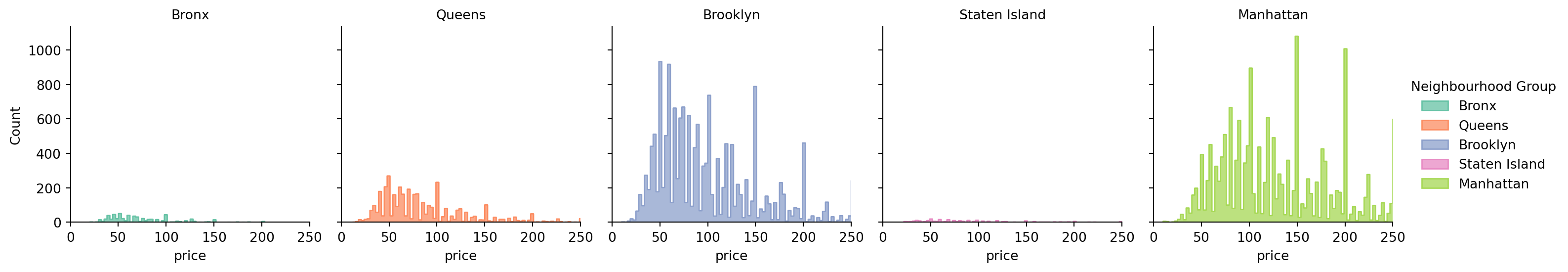

Average prices by room type:

# Group by room_type and calculate mean price
mean_price_by_room = round(nyc_airbnb.groupby('room_type')['price'].mean(),2).reset_index()
print(mean_price_by_room)

         room_type   price
0  Entire home/apt  206.63
1     Private room   87.52
2      Shared room   70.20

Median prices by room type by neighborhood:

# Group by neighbourhood_group and room_type, compute median price, and pivot the table
median_price_pivot = nyc_airbnb.groupby(['neighbourhood_group', 'room_type'])['price'].median().unstack()
print(median_price_pivot)

room_type            Entire home/apt  Private room  Shared room
neighbourhood_group                                            
Bronx                          100.0          55.0         43.0
Brooklyn                       145.0          65.0         40.0
Manhattan                      190.0          90.0         65.0
Queens                         119.0          60.0         39.0
Staten Island                  112.5          55.0         25.0

Review scores’ affect on prices:

# Scatter plot of review_scores_location vs price
plt.figure(figsize=(10, 6))
sns.scatterplot(data=nyc_airbnb, x='review_scores_location', y='price')
plt.xlabel('Review Scores')
plt.ylabel('Price')
plt.show()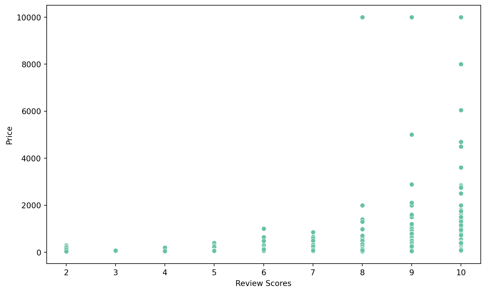

Does room type affect availabilities?

Now, we explore the relation between room types and availabilities. A violin plot is similar to a boxplot, with the exception of a rotated kernel density plot on each side.

# Violin plot of room_type vs availability_365
# Set cut = 0 to restrict violin plot within min-max range. Otherwise, default = 2 which extends the density past extreme datapoints
plt.figure(figsize=(10, 6))
sns.violinplot(data=nyc_airbnb, x='room_type', y='availability_365', cut = 0)
plt.xlabel('Room Type')
plt.ylabel('Days available in a year')
plt.show()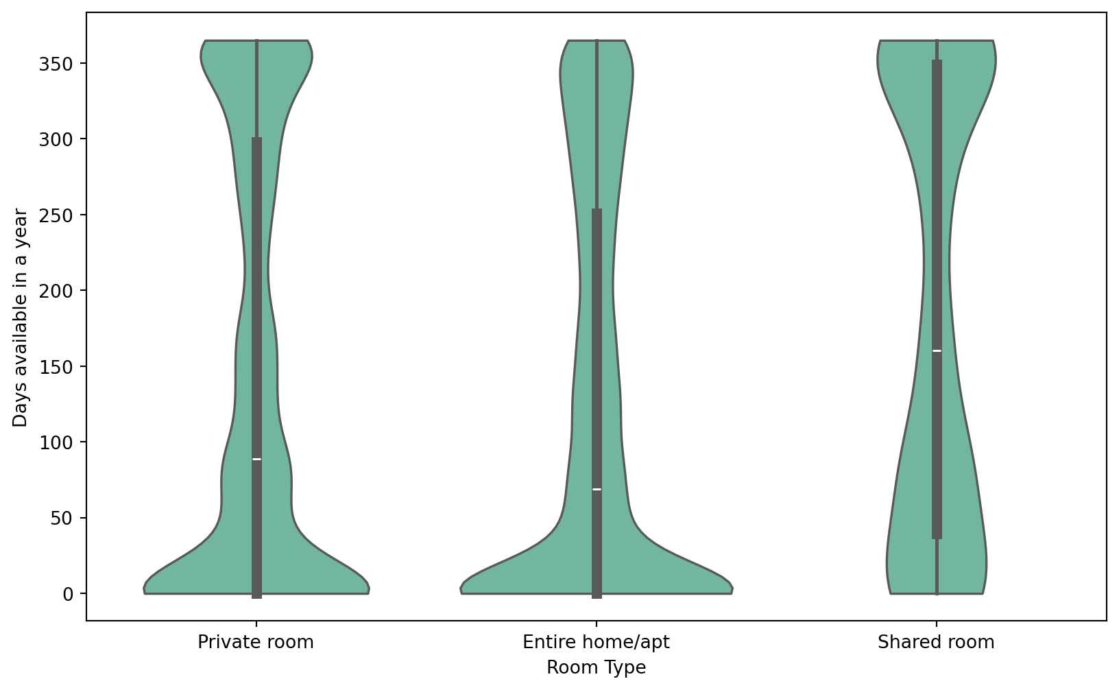

What about reviews and popularity?

Number of reviews by neighborhood:

# Group by neighbourhood_group and sum number_of_reviews, then sort
reviews_by_group = nyc_airbnb.groupby('neighbourhood_group')['number_of_reviews'].sum()\
                    .reset_index().sort_values(by='number_of_reviews', ascending=False)
print(reviews_by_group)

  neighbourhood_group  number_of_reviews
2           Manhattan             323941
1            Brooklyn             263542
3              Queens              66611
0               Bronx               9897
4       Staten Island               4744

Relationship between number of reviews and the review scores:

# Scatter plot of number_of_reviews vs review_scores_location
plt.figure(figsize=(10, 6))
sns.scatterplot(data=nyc_airbnb, x='number_of_reviews', y='review_scores_location')
plt.xlabel('Number of Reviews')
plt.ylabel('Review Scores')
plt.show()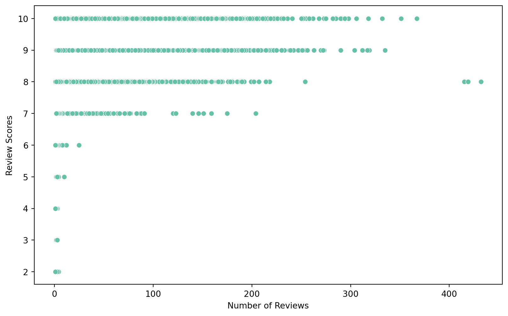

Repeated hosts?

# Filter hosts with multiple calculated listings
filtered_hosts = nyc_airbnb[nyc_airbnb['calculated_host_listings_count'] > 34]
filtered_hosts.head()

	id	review_scores_location	name	host_id	host_name	neighbourhood_group	neighbourhood	long	lat	room_type	price	minimum_nights	number_of_reviews	last_review	reviews_per_month	calculated_host_listings_count	availability_365
1589	15057686	NaN	Home 4 Medical Professionals- Stuyvesant Heigh...	26377263	Stat	Brooklyn	Bedford-Stuyvesant	-73.950457	40.687853	Private room	54	30	0	NaN	NaN	35	289
1810	15080936	NaN	Home 4 Medical Professionals- Stuyvesant Heigh...	26377263	Stat	Brooklyn	Bedford-Stuyvesant	-73.950478	40.689792	Private room	57	30	0	NaN	NaN	35	264
2897	14776203	10.0	Home 4 Medical Professionals- Stuyvesant Heigh...	26377263	Stat	Brooklyn	Bedford-Stuyvesant	-73.952462	40.687926	Private room	57	30	1	2/18/17	0.39	35	362
4288	15074005	NaN	Home 4 Medical Professionals- Stuyvesant Heigh...	26377263	Stat	Brooklyn	Bedford-Stuyvesant	-73.951861	40.689432	Private room	54	30	0	NaN	NaN	35	320
4540	5866656	NaN	Home 4 Medical Professionals-MAIM0	26377263	Stat	Brooklyn	Borough Park	-73.997281	40.640318	Private room	50	30	0	NaN	NaN	35	355

Now, let’s do a deeper dive in Manhattan.

We take a closer look in Manhattan. We only limit our search to those whose prices are under $1000.

# Manhattan listings with price < 1000 mapped by latitude and longitude
manhattan_filtered = nyc_airbnb[(nyc_airbnb['neighbourhood_group'] == 'Manhattan') & (nyc_airbnb['price'] < 1000)]
plt.figure(figsize=(8, 6))
sns.scatterplot(data=manhattan_filtered, x='lat', y='long', hue='price',size='price', alpha=0.7)
plt.xlabel('Latitude')
plt.ylabel('Longitude')
plt.legend(title='Price by $')
plt.show()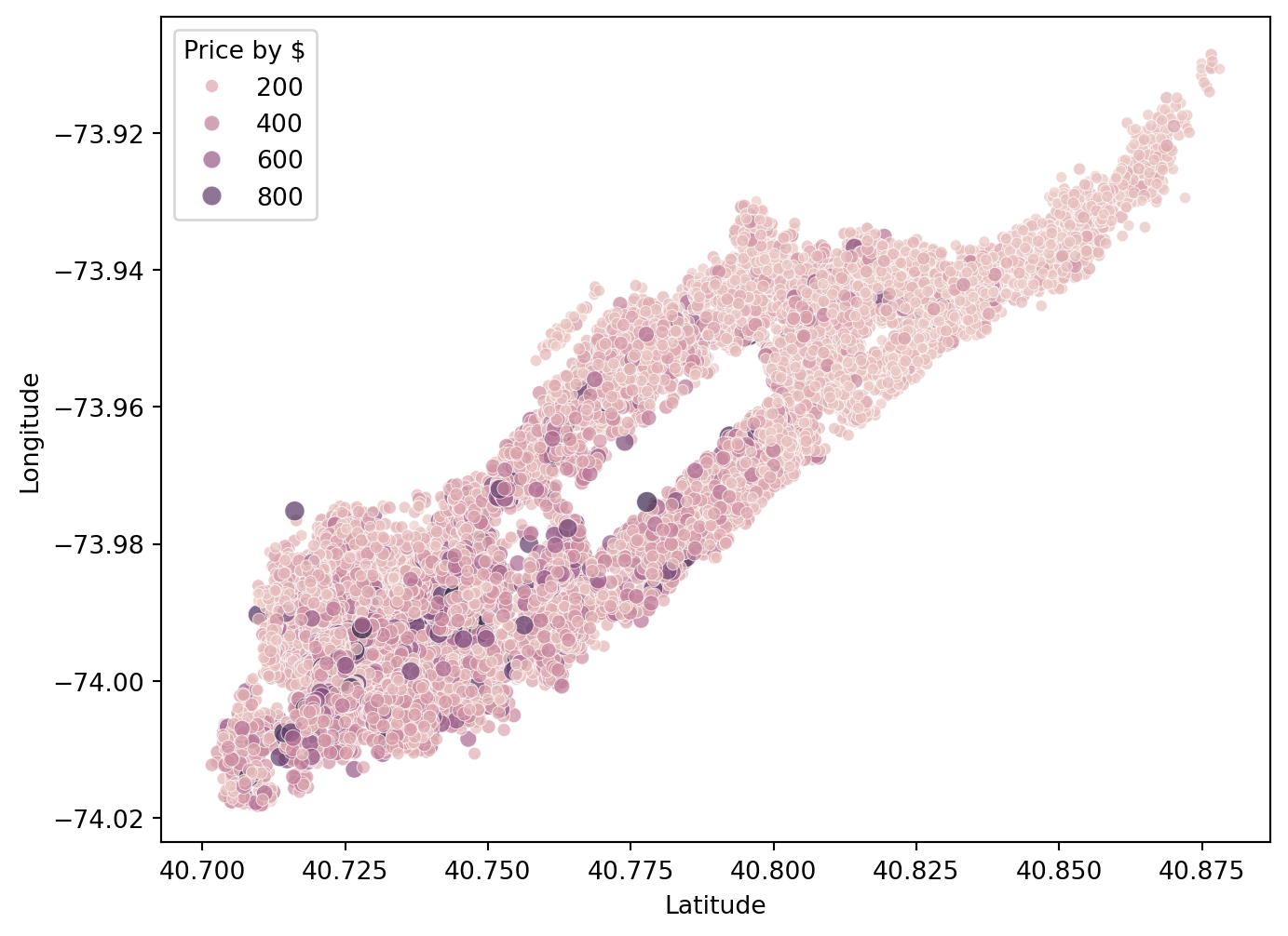

Let’s see what the average prices for entire homes under $1000 are, in each Manhattan neighborhood:

# Compute mean price by neighbourhood for Manhattan entire homes under $1000
manhattan_entire_home = manhattan_filtered[manhattan_filtered['room_type'] == 'Entire home/apt']
mean_price_neighbourhood = manhattan_entire_home.groupby('neighbourhood')['price'].mean().reset_index().sort_values(by='price', ascending=False)
print(mean_price_neighbourhood)

          neighbourhood       price
26              Tribeca  358.030000
20                 NoHo  311.573770
7     Flatiron District  306.840000
23                 SoHo  295.735043
25     Theater District  282.193548
17              Midtown  275.967939
0     Battery Park City  270.659091
9     Greenwich Village  255.833333
1               Chelsea  254.603922
6    Financial District  249.907895
11       Hell's Kitchen  246.286866
31         West Village  245.414356
21               Nolita  241.170732
14         Little Italy  237.829787
13             Kips Bay  227.217712
19          Murray Hill  226.341615
29      Upper West Side  223.983271
24      Stuyvesant Town  223.071429
3          Civic Center  218.880000
8              Gramercy  214.566667
5          East Village  210.396313
2             Chinatown  207.256410
15      Lower East Side  204.777778
28      Upper East Side  192.833167
27          Two Bridges  173.761905
10               Harlem  164.489627
4           East Harlem  163.313225
18  Morningside Heights  150.707006
30   Washington Heights  132.896154
22     Roosevelt Island  130.875000
12               Inwood  119.079545
16          Marble Hill  100.833333

# Violin plot of price by Manhattan neighbourhood, reordered by price
plt.figure(figsize=(14, 5))
manhattan_entire_home_sorted = manhattan_entire_home.sort_values(by='price')
sns.violinplot(data=manhattan_entire_home_sorted, x='neighbourhood', y='price')
plt.xticks(rotation=45,ha="right", rotation_mode="anchor")
plt.show()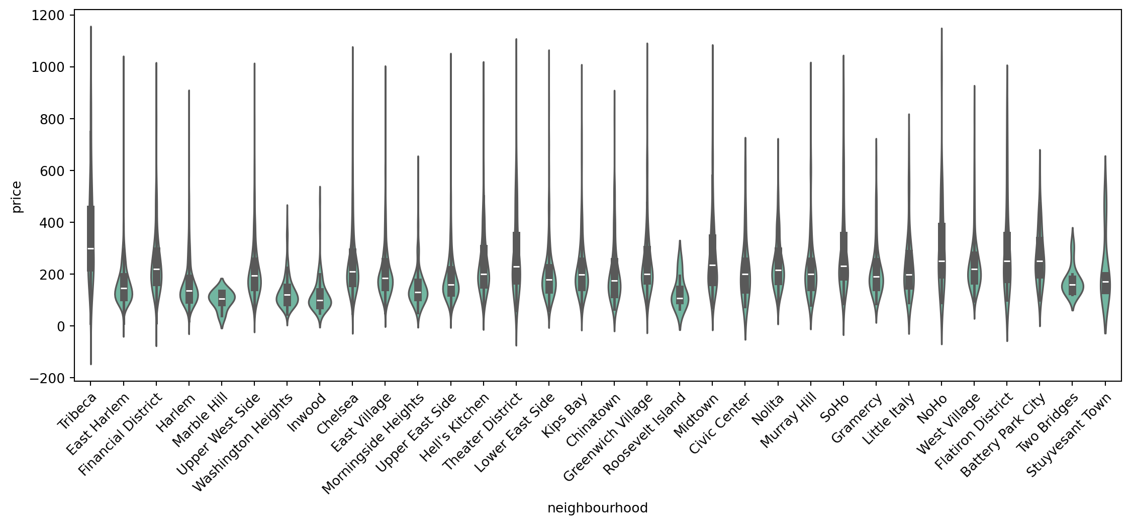

# drop nas from review
manhattan_filtered_dropna = manhattan_filtered.dropna(subset='review_scores_location')

fig = px.scatter_map(
    manhattan_filtered_dropna,
    lon='long',
    lat='lat',
    opacity=0.6,
    color='review_scores_location',
    color_continuous_scale=px.colors.sequential.Viridis,
    labels={"review_scores_location": "Review Score"}
)

fig.update_layout(
    autosize=False, height=500, width=800,
    title=dict(text="AirBnB Review Scores in Manhattan")
)


fig.show()

Case Study: Food Prices for Nutrition

The Food Prices for Nutrition data set is taken from Word Bank Group International Comparison Program (ICP). It records costs and affordabilities of various diets across different countries from 2017 to 2022. You can check the summary and some basic analyses of this data set through its website in the link before. In this case study, we will take a dive into this data set and do some exploratory data analysis.

What does the data look like?

Before we ask any scientific question about the data set, we need to at least take a look at it!

df = pd.read_csv("../data/food_prices.csv")

df.head()

	Classification Name	Classification Code	Country Name	Country Code	Time	Time Code	Cost of an energy sufficient diet [CoCA]	Cost of a nutrient adequate diet [CoNA]	Cost of a healthy diet [CoHD]	Cost of a healthy diet relative to the cost of sufficient energy from starchy staples [CoHD_CoCA]	...	Affordability of an energy sufficient diet: ratio of cost to food expenditures [CoCA_fexp]	Affordability of a nutrient adequate diet: ratio of cost to food expenditures [CoNA_fexp]	Affordability of a healthy diet: ratio of cost to food expenditures [CoHD_fexp]	Percent of the population who cannot afford sufficient calories [CoCA_headcount]	Percent of the population who cannot afford nutrient adequacy [CoNA_headcount]	Percent of the population who cannot afford a healthy diet [CoHD_headcount]	Millions of people who cannot afford sufficient calories [CoCA_unafford_n]	Millions of people who cannot afford nutrient adequacy [CoNA_unafford_n]	Millions of people who cannot afford a healthy diet [CoHD_unafford_n]	Population [Pop]
0	Food Prices for Nutrition 1.0	FPN 1.0	Albania	ALB	2017.0	YR2017	0.725	2.471	3.952	5.45	...	0.078	0.266	0.425	0	13	37.8	0	0.4	1.1	2873457
1	Food Prices for Nutrition 1.0	FPN 1.0	Albania	ALB	2018.0	YR2018	..	..	4.051	..	...	..	..	..	..	..	27.9	..	..	0.8	2866376
2	Food Prices for Nutrition 1.0	FPN 1.0	Albania	ALB	2019.0	YR2019	..	..	4.117	..	...	..	..	..	..	..	19.8	..	..	0.6	2854191
3	Food Prices for Nutrition 1.0	FPN 1.0	Albania	ALB	2020.0	YR2020	..	..	4.197	..	...	..	..	..	..	..	20.1	..	..	0.6	2837743
4	Food Prices for Nutrition 1.0	FPN 1.0	Albania	ALB	2021.0	YR2021	..	..	..	..	...	..	..	..	..	..	..	..	..	..	..

5 rows × 40 columns

The countries included in this program.

df['Country Name'].unique()

array(['Albania', 'Algeria', 'Angola', 'Anguilla', 'Antigua and Barbuda',
       'Argentina', 'Armenia', 'Aruba', 'Australia', 'Austria',
       'Azerbaijan', 'Bahamas, The', 'Bahrain', 'Bangladesh', 'Barbados',
       'Belarus', 'Belgium', 'Belize', 'Benin', 'Bermuda', 'Bhutan',
       'Bolivia', 'Bonaire', 'Bosnia and Herzegovina', 'Botswana',
       'Brazil', 'British Virgin Islands', 'Brunei Darussalam',
       'Bulgaria', 'Burkina Faso', 'Burundi', 'Cabo Verde', 'Cambodia',
       'Cameroon', 'Canada', 'Cayman Islands', 'Central African Republic',
       'Chad', 'Chile', 'China', 'Colombia', 'Comoros',
       'Congo, Dem. Rep.', 'Congo, Rep.', 'Costa Rica', "Côte d'Ivoire",
       'Croatia', 'Curacao', 'Cyprus', 'Czech Republic', 'Denmark',
       'Djibouti', 'Dominica', 'Dominican Republic',
       'East Asia & Pacific', 'Ecuador', 'Egypt, Arab Rep.',
       'El Salvador', 'Equatorial Guinea', 'Estonia', 'Eswatini',
       'Ethiopia', 'Europe & Central Asia', 'Fiji', 'Finland', 'France',
       'Gabon', 'Gambia, The', 'Germany', 'Ghana', 'Greece', 'Grenada',
       'Guinea', 'Guinea-Bissau', 'Guyana', 'Haiti', 'High income',
       'Honduras', 'Hong Kong SAR, China', 'Hungary', 'Iceland', 'India',
       'Indonesia', 'Iran, Islamic Rep.', 'Iraq', 'Ireland', 'Israel',
       'Italy', 'Jamaica', 'Japan', 'Jordan', 'Kazakhstan', 'Kenya',
       'Korea, Rep.', 'Kuwait', 'Kyrgyz Republic', 'Lao PDR',
       'Latin America & Caribbean', 'Latvia', 'Lesotho', 'Liberia',
       'Lithuania', 'Low income', 'Lower middle income', 'Luxembourg',
       'Madagascar', 'Malawi', 'Malaysia', 'Maldives', 'Mali', 'Malta',
       'Mauritania', 'Mauritius', 'Mexico', 'Middle East & North Africa',
       'Moldova', 'Mongolia', 'Montenegro', 'Montserrat', 'Morocco',
       'Mozambique', 'Myanmar', 'Namibia', 'Nepal', 'Netherlands',
       'New Zealand', 'Nicaragua', 'Niger', 'Nigeria', 'North America',
       'North Macedonia', 'Norway', 'Oman', 'Pakistan', 'Panama',
       'Paraguay', 'Peru', 'Philippines', 'Poland', 'Portugal', 'Qatar',
       'Romania', 'Russian Federation', 'Rwanda', 'Sao Tome and Principe',
       'Saudi Arabia', 'Senegal', 'Serbia', 'Seychelles', 'Sierra Leone',
       'Singapore', 'Sint Maarten (Dutch part)', 'Slovak Republic',
       'Slovenia', 'South Africa', 'South Asia', 'Spain', 'Sri Lanka',
       'St. Kitts and Nevis', 'St. Lucia',
       'St. Vincent and the Grenadines', 'Sub-Saharan Africa', 'Sudan',
       'Suriname', 'Sweden', 'Switzerland', 'Taiwan, China', 'Tajikistan',
       'Tanzania', 'Thailand', 'Togo', 'Trinidad and Tobago', 'Tunisia',
       'Türkiye', 'Turks and Caicos Islands', 'Uganda',
       'United Arab Emirates', 'United Kingdom', 'United States',
       'Upper middle income', 'Uruguay', 'Vietnam', 'West Bank and Gaza',
       'WORLD', 'Zambia', 'Zimbabwe', nan], dtype=object)

The number of records and the number of variables.

df.shape

(3725, 40)

Let’s look at the variables:

df.columns

Index(['Classification Name', 'Classification Code', 'Country Name',
       'Country Code', 'Time', 'Time Code',
       'Cost of an energy sufficient diet [CoCA]',
       'Cost of a nutrient adequate diet [CoNA]',
       'Cost of a healthy diet [CoHD]',
       'Cost of a healthy diet relative to the cost of sufficient energy from starchy staples [CoHD_CoCA]',
       'Cost of fruits [CoHD_f]', 'Cost of vegetables [CoHD_v]',
       'Cost of starchy staples [CoHD_ss]',
       'Cost of animal-source foods [CoHD_asf]',
       'Cost of legumes, nuts and seeds [CoHD_lns]',
       'Cost of oils and fats [CoHD_of]',
       'Cost share for fruits in a least-cost healthy diet [CoHD_f_prop]',
       'Cost share for vegetables in a least-cost healthy diet [CoHD_v_prop]',
       'Cost share for starchy staples in a least-cost healthy diet [CoHD_ss_prop]',
       'Cost share for animal-sourced foods in a least-cost healthy diet [CoHD_asf_prop]',
       'Cost share for legumes, nuts and seeds in a least-cost healthy diet [CoHD_lns_prop]',
       'Cost share for oils and fats in a least-cost healthy diet [CoHD_of_prop]',
       'Cost of fruits relative to the starchy staples in a least-cost healthy diet [CoHD_f_ss]',
       'Cost of vegetables relative to the starchy staples in a least-cost healthy diet [CoHD_v_ss]',
       'Cost of animal-sourced foods relative to the starchy staples in a least-cost healthy diet [CoHD_asf_ss]',
       'Cost of legumes, nuts and seeds relative to the starchy staples in a least-cost healthy diet [CoHD_lns_ss]',
       'Cost of oils and fats relative to the starchy staples in a least-cost healthy diet [CoHD_of_ss]',
       'Affordability of an energy sufficient diet: ratio of cost to the food poverty line [CoCA_pov]',
       'Affordability of a nutrient adequate diet: ratio of cost to the food poverty line [CoNA_pov]',
       'Affordability of a healthy diet: ratio of cost to the food poverty line [CoHD_pov]',
       'Affordability of an energy sufficient diet: ratio of cost to food expenditures [CoCA_fexp]',
       'Affordability of a nutrient adequate diet: ratio of cost to food expenditures [CoNA_fexp]',
       'Affordability of a healthy diet: ratio of cost to food expenditures [CoHD_fexp]',
       'Percent of the population who cannot afford sufficient calories [CoCA_headcount]',
       'Percent of the population who cannot afford nutrient adequacy [CoNA_headcount]',
       'Percent of the population who cannot afford a healthy diet [CoHD_headcount]',
       'Millions of people who cannot afford sufficient calories [CoCA_unafford_n]',
       'Millions of people who cannot afford nutrient adequacy [CoNA_unafford_n]',
       'Millions of people who cannot afford a healthy diet [CoHD_unafford_n]',
       'Population [Pop]'],
      dtype='object')

Data Cleaning

We need to process the data to a format that we can easily manipulate.

df.dropna(inplace = True)
selected_countries = ["India", "Senegal", "Albania", "China", "United States", "United Arab Emirates", "Türkiye", "Egypt, Arab Rep.", "Ghana"]
df = df[df['Country Name'].isin(selected_countries)]

df.head()

	Classification Name	Classification Code	Country Name	Country Code	Time	Time Code	Cost of an energy sufficient diet [CoCA]	Cost of a nutrient adequate diet [CoNA]	Cost of a healthy diet [CoHD]	Cost of a healthy diet relative to the cost of sufficient energy from starchy staples [CoHD_CoCA]	...	Affordability of an energy sufficient diet: ratio of cost to food expenditures [CoCA_fexp]	Affordability of a nutrient adequate diet: ratio of cost to food expenditures [CoNA_fexp]	Affordability of a healthy diet: ratio of cost to food expenditures [CoHD_fexp]	Percent of the population who cannot afford sufficient calories [CoCA_headcount]	Percent of the population who cannot afford nutrient adequacy [CoNA_headcount]	Percent of the population who cannot afford a healthy diet [CoHD_headcount]	Millions of people who cannot afford sufficient calories [CoCA_unafford_n]	Millions of people who cannot afford nutrient adequacy [CoNA_unafford_n]	Millions of people who cannot afford a healthy diet [CoHD_unafford_n]	Population [Pop]
0	Food Prices for Nutrition 1.0	FPN 1.0	Albania	ALB	2017.0	YR2017	0.725	2.471	3.952	5.45	...	0.078	0.266	0.425	0	13	37.8	0	0.4	1.1	2873457
1	Food Prices for Nutrition 1.0	FPN 1.0	Albania	ALB	2018.0	YR2018	..	..	4.051	..	...	..	..	..	..	..	27.9	..	..	0.8	2866376
2	Food Prices for Nutrition 1.0	FPN 1.0	Albania	ALB	2019.0	YR2019	..	..	4.117	..	...	..	..	..	..	..	19.8	..	..	0.6	2854191
3	Food Prices for Nutrition 1.0	FPN 1.0	Albania	ALB	2020.0	YR2020	..	..	4.197	..	...	..	..	..	..	..	20.1	..	..	0.6	2837743
4	Food Prices for Nutrition 1.0	FPN 1.0	Albania	ALB	2021.0	YR2021	..	..	..	..	...	..	..	..	..	..	..	..	..	..	..

5 rows × 40 columns

cost_of_diet, percent_cannot_afford = "Cost of a healthy diet [CoHD]", "Percent of the population who cannot afford a healthy diet [CoHD_headcount]"
df = df[["Country Name", cost_of_diet,  "Classification Code", "Time", "Population [Pop]", percent_cannot_afford]]
df = df.replace("..", pd.NA)
df = df.dropna()

df = df[df["Classification Code"] == "FPN 2.1"]
df['Time'] = df['Time'].astype(int)
df['Country Name'] = df['Country Name'].astype(str)
df['Population [Pop]'] = df['Population [Pop]'].astype(int)
df[percent_cannot_afford] = df[percent_cannot_afford].astype(float)
df[cost_of_diet] = df[cost_of_diet].astype(float)

df = df.drop_duplicates()
df = df.drop(columns = ["Classification Code"])

df.dtypes

Country Name                                                                    object
Cost of a healthy diet [CoHD]                                                  float64
Time                                                                             int64
Population [Pop]                                                                 int64
Percent of the population who cannot afford a healthy diet [CoHD_headcount]    float64
dtype: object

df.head()

	Country Name	Cost of a healthy diet [CoHD]	Time	Population [Pop]	Percent of the population who cannot afford a healthy diet [CoHD_headcount]
2790	Albania	3.952	2017	2873457	31.3
2791	Albania	4.069	2018	2866376	23.0
2792	Albania	4.262	2019	2854191	22.2
2793	Albania	4.280	2020	2837849	19.9
2794	Albania	4.388	2021	2811666	15.7

The population is at a very large scale, so usually we need to trasform it to log scale for better visualization, etc.

df["pop_log"] = np.log(df["Population [Pop]"])

df.head()

	Country Name	Cost of a healthy diet [CoHD]	Time	Population [Pop]	Percent of the population who cannot afford a healthy diet [CoHD_headcount]	pop_log
2790	Albania	3.952	2017	2873457	31.3	14.871026
2791	Albania	4.069	2018	2866376	23.0	14.868559
2792	Albania	4.262	2019	2854191	22.2	14.864299
2793	Albania	4.280	2020	2837849	19.9	14.858557
2794	Albania	4.388	2021	2811666	15.7	14.849288

Interactive Scatter Plot

# Create an interactive scatter plot with a slider using Plotly Express
fig = px.scatter(
    df,
    x='Cost of a healthy diet [CoHD]',
    y='Percent of the population who cannot afford a healthy diet [CoHD_headcount]',
    size='pop_log',
    animation_frame='Time',  
    color = 'Country Name',
    title='Cost of diet Vs % of population who cannot afford it through the years',
    labels={'Population [Pop]': 'Point Size'}
)

fig.update_xaxes(range=[2, 4.5])  # Adjust the range based on your desired x-axis limits
fig.update_yaxes(range=[-10, 100])  

fig.update_layout(
    title_x=0.5,  # Center the title
    yaxis_title="% cannot afford",
    xaxis_title='Cost of a Healthy Diet',
    height=600, width=800,
)

# Show the interactive plot
fig.show()