Lecture 12 - Big data and databases

Overview

In this lecture, we discuss computing issues that arise with big data, and potential solutions including:

• pandas chunking
• sqlite
• duckdb
• polars

References

• Python for Data Analysis (Wes McKinney, 2022)
• DuckDB tutorial
• Modern Polars (Kevin Heavey, 2024)

Computing and big data issues

Simply put, a computer is made up of three basic parts:

• the memory units (e.g. random access memory, RAM; solid-state drive, SSD)
• the computing units (e.g. central processing unit, CPU; graphics processing unit, GPU)
• the connections between them

Memory

RAM	Solid-state drive
Temporary memory used for actively running programs/data	Permanent storage for your operating system, applications, and files
Extremely fast read/write	Slower read/write
Smaller (typically 8-64 GB)	Larger (TBs)

If a dataset is loaded into RAM, we typically say it is “in memory”

If a dataset is on the solid-state drive, we typically say it is “on disk”.

Compute

CPU	GPU
General-purpose processor	Highly parallel processor for repetitive tasks (originally for graphics)
Few cores (e.g. 4–32)	Thousands of smaller cores
Strong per-core performance	Weak individual cores, but excellent at parallel tasks
Ideal for logic-heavy tasks, branching, single-thread performance	Ideal for matrix operations, linear algebra, deep learning

Issues

Pandas in particular struggles with big data due to:

• memory: pandas loads the entire dataset into RAM. As RAM is on the order of GB, this is problematic for datasets of that size.

• compute: pandas typically takes advantage of only one CPU core, unlike other libraries which parallelize operations to multiple cores under the hood. For large data, this means pandas operations can be much slower than other libraries.

• eager evaluation: pandas uses eager evaluation, which means it executes computations immediately when invoked. Other libraries use lazy evaluation, where computations are only run when needed. Lazy evaluation is often optimized to avoid unnecessary computations, and not store intermediate calculations.

Pandas and big data

There are a few things we can do in pandas to help with memory issues:

• subsetting columns: load in only a subset of columns at a time
• chunking: load in only a few rows at a time

Subsetting columns

import pandas as pd

head_df = pd.read_csv('../data/rates.csv', nrows=0)

head_df.columns

Index(['Time', 'USD', 'JPY', 'BGN', 'CZK', 'DKK', 'GBP', 'CHF'], dtype='object')

rates_df = pd.read_csv('../data/rates.csv', usecols=head_df.columns[:3])

rates_df.head()

	Time	USD	JPY
0	2024-04-16	1.0637	164.54
1	2024-04-15	1.0656	164.05
2	2024-04-12	1.0652	163.16
3	2024-04-11	1.0729	164.18
4	2024-04-10	1.0860	164.89

Chunking

The function pd.read_csv has an optional argument chunksize.

When you specify chunksize, pd.read_csv returns an iterable instead of a DataFrame. To access the chunks of data, iterate over the iterable.

Let’s consider this dataset from Kaggle of over 900K songs.

# get header
spotify_header = pd.read_csv("../data/spotify_dataset.csv", nrows=0)

spotify_header.columns

Index(['Artist(s)', 'song', 'text', 'Length', 'emotion', 'Genre', 'Album',
       'Release Date', 'Key', 'Tempo', 'Loudness (db)', 'Time signature',
       'Explicit', 'Popularity', 'Energy', 'Danceability', 'Positiveness',
       'Speechiness', 'Liveness', 'Acousticness', 'Instrumentalness',
       'Good for Party', 'Good for Work/Study',
       'Good for Relaxation/Meditation', 'Good for Exercise',
       'Good for Running', 'Good for Yoga/Stretching', 'Good for Driving',
       'Good for Social Gatherings', 'Good for Morning Routine',
       'Similar Artist 1', 'Similar Song 1', 'Similarity Score 1',
       'Similar Artist 2', 'Similar Song 2', 'Similarity Score 2',
       'Similar Artist 3', 'Similar Song 3', 'Similarity Score 3'],
      dtype='object')

chunk_iter = pd.read_csv("../data/spotify_dataset.csv", chunksize=1000)

chunk = next(chunk_iter)

chunk['Genre'].unique()

array(['hip hop', 'jazz', 'indie rock,britpop', 'classical',
       'rock,pop,comedy', 'rock,pop rock', 'rap,hip hop',
       'trance,electronic,psychedelic', 'country,classic rock,hard rock',
       'hip hop,trap,cloud rap', 'electronic,rap',
       'rock,hardcore,garage rock', 'pop',
       'chillout,psychedelic,electronic', 'alternative rock,new wave',
       'hip-hop,hip hop', 'punk,punk rock', 'k-pop',
       'metal,hard rock,heavy metal', 'rock,synthpop,alternative rock',
       'country,pop', 'folk', 'alternative rock,indie rock,indie', 'rock'],
      dtype=object)

chunk_iter = pd.read_csv("../data/spotify_dataset.csv", chunksize=1000)
result = []

for chunk in chunk_iter:
    chunk['genre_1'] = chunk['Genre'].str.split(',').str[0]
    group = chunk.groupby("genre_1")["Danceability"].agg(['sum', 'count'])
    result.append(group)

final = pd.concat(result).reset_index()

final['genre_1'] = final['genre_1'].str.replace('hip hop', 'hip-hop')

final = final.groupby("genre_1").sum()
final = final.reset_index()

total_songs = final['count'].sum()

final.rename(columns={'genre_1': 'Genre', 'sum': 'Danceability'}, inplace=True)

final = final[final['count'] > 1000]

final['Danceability'] = final['Danceability'] / final['count']

import seaborn as sns
import matplotlib.pyplot as plt

sns.stripplot(final.sort_values(by='Danceability', ascending=False),
              x='Danceability',
              y='Genre')
plt.gca().xaxis.grid(False)
plt.gca().yaxis.grid(True)
plt.gcf().set_size_inches(5, 8)
plt.gca().set(xlim=(0, 76), title='Danceability by Genre', xlabel="", ylabel="");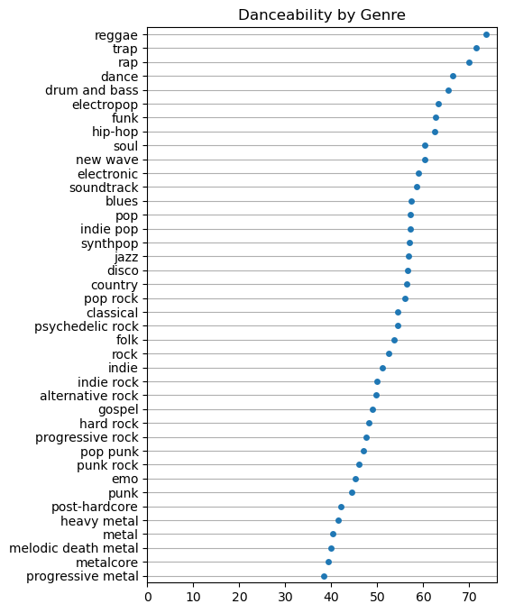

Other Pandas tips

• Chain commands instead of doing step-by-step

Example:

# DO THIS
group = chunk.groupby("genre_1")["Danceability"].agg(['sum', 'count'])

# NOT THIS
group = chunk.groupby("genre_1")
dance = group["Danceability"].agg(['sum', 'count'])

• Use categoricals instead of strings

Databases

Much of this section is drawn from Software Carpentry.

Databases can handle large, complex datasets. Databases include powerful tools for search and analysis, without loading the data into memory.

Relational databases

A relational database is a way to store and manipulate information.

The data is stored in objects called tables. Tables have:

• columns (also known as fields)
• rows (also known as records)

The database is “relational” in that the tables are connected in some way. For example, one table may be a list of customers and their characteristics; another table may be customer transactions.

Querying databases

When we use a database, we send commands - usually called queries - to a database manager: a program that manipulates the database for us.

Queries are written in a language called SQL, which stands for “Structured Query Language”. SQL commands fall into the “CRUD” categories:

• Create: e.g. CREATE, INSERT
• Read: e.g. SELECT
• Update: e.g. UPDATE
• Delete: e.g. DELETE, DROP

SQLite

We introduce the basics of SQL using SQLite.

SQLite is a server-less, open-source database management system.

SQLite can handle data of even hundreds or thousands of gigabytes in size that fit on a single computer’s disk.

In Python, sqlite3 is a built-in library.

Connecting to a database

We work with the database survey.db, downloaded from here.

The database contains data from an expedition to the Pole of Inaccessbility in the South Pacific and Antarctica in the late 1920s and early 1930s. The expedition was led by William Dyer, Frank Pabodie, and Valentina Roerich.

• Open a connection to a database using sqlite3.connect()

Note

If the database does not exist, sqlite will create a new database with that name.

import sqlite3

conn = sqlite3.connect("../data/survey.db")

The returned Connection object conn represents the connection to the on-disk database.

To execute SQL statement and fetch results from SQL queries to the database, we need a database cursor.

• call conn.cursor() to create the Cursor:

cursor = conn.cursor()

Schema

What does the database contain?

Every SQLite database contains a single schema table that stores the schema (or description) for that database.

The schema is a description of all the tables, indexes, triggers and views (collectively “objects”) that are contained within the database.

The sqlite_schema table contains:

• one row for each object in the schema

• the columns include:

  • type: one of ‘table’, ‘index’, ‘view’ or ‘trigger’
  • name: name of object
  • sql: SQL text that describes the object

  (for full column list, see docs).

Querying the schema

We can use a SQL query to inspect the schema:

SELECT name, sql FROM sqlite_schema

• SELECT defines which columns to return
• FROM defines the source table

cursor.execute("SELECT name, sql FROM sqlite_schema")
tables = cursor.fetchall()

for tab in tables:
    print(tab)

('Person', 'CREATE TABLE Person (id text, personal text, family text)')
('Site', 'CREATE TABLE Site (name text, lat real, long real)')
('Survey', 'CREATE TABLE Survey (taken integer, person text, quant text, reading real)')
('Visited', 'CREATE TABLE Visited (id integer, site text, dated text)')

Consider the first line. The sql column tells us that the table Person has three columns:

• id with type text
• personal with type text
• family with type text

Selecting

Now we know what is in our database, let’s look at the tables.

We can select all columns in a table using *:

cursor.execute("SELECT * FROM Person")
rows = cursor.fetchall()
cols = [description[0] for description in cursor.description]

pd.DataFrame(rows, columns=cols)

	id	personal	family
0	dyer	William	Dyer
1	pb	Frank	Pabodie
2	lake	Anderson	Lake
3	roe	Valentina	Roerich
4	danforth	Frank	Danforth

cursor.execute("SELECT * FROM Site")
rows = cursor.fetchall()
cols = [description[0] for description in cursor.description]

pd.DataFrame(rows, columns=cols)

	name	lat	long
0	DR-1	-49.85	-128.57
1	DR-3	-47.15	-126.72
2	MSK-4	-48.87	-123.40

We can also count how many rows there are in a table.

cursor.execute("SELECT COUNT(*) FROM Visited")
rows = cursor.fetchall()
cols = [description[0] for description in cursor.description]

pd.DataFrame(rows, columns=cols)

	COUNT(*)
0	8

cursor.execute("SELECT * FROM Visited")
rows = cursor.fetchall()
cols = [description[0] for description in cursor.description]

pd.DataFrame(rows, columns=cols).head()

	id	site	dated
0	619	DR-1	1927-02-08
1	622	DR-1	1927-02-10
2	734	DR-3	1930-01-07
3	735	DR-3	1930-01-12
4	751	DR-3	1930-02-26

cursor.execute("SELECT COUNT(*) FROM Survey")
rows = cursor.fetchall()
cols = [description[0] for description in cursor.description]

pd.DataFrame(rows, columns=cols)

	COUNT(*)
0	21

cursor.execute("SELECT * FROM Survey")
rows = cursor.fetchall()
cols = [description[0] for description in cursor.description]

pd.DataFrame(rows, columns=cols).head()

	taken	person	quant	reading
0	619	dyer	rad	9.82
1	619	dyer	sal	0.13
2	622	dyer	rad	7.80
3	622	dyer	sal	0.09
4	734	pb	rad	8.41

We can also select and order at the same time.

cursor.execute("SELECT * FROM Person ORDER BY id")
rows = cursor.fetchall()
cols = [description[0] for description in cursor.description]

pd.DataFrame(rows, columns=cols)

	id	personal	family
0	danforth	Frank	Danforth
1	dyer	William	Dyer
2	lake	Anderson	Lake
3	pb	Frank	Pabodie
4	roe	Valentina	Roerich

To do descending order, use

SELECT * FROM Person ORDER BY id DESC

Now, suppose we want to know what are different types of quantities (quant) collected. We can use the keyword DISTINCT.

cursor.execute("SELECT DISTINCT quant FROM Survey")
rows = cursor.fetchall()
cols = [description[0] for description in cursor.description]

pd.DataFrame(rows, columns=cols).head()

	quant
0	rad
1	sal
2	temp

If we want to determine which visit (stored in the taken column) have which quant measurement, we can use the DISTINCT keyword on multiple columns.

cursor.execute("SELECT DISTINCT taken, quant FROM Survey")
rows = cursor.fetchall()
cols = [description[0] for description in cursor.description]

pd.DataFrame(rows, columns=cols)

	taken	quant
0	619	rad
1	619	sal
2	622	rad
3	622	sal
4	734	rad
5	734	sal
6	734	temp
7	735	rad
8	735	sal
9	735	temp
10	751	rad
11	751	temp
12	751	sal
13	752	rad
14	752	sal
15	752	temp
16	837	rad
17	837	sal
18	844	rad

In order to look at which scientist measured quantities during each visit, we can look again at the Survey table.

This query sorts results first by taken, and then by person within each group of equal taken values:

cursor.execute("""
            SELECT taken, person, quant 
            FROM Survey 
            ORDER BY taken , person
""")
    
rows = cursor.fetchall()
cols = [description[0] for description in cursor.description]

pd.DataFrame(rows, columns=cols)

	taken	person	quant
0	619	dyer	rad
1	619	dyer	sal
2	622	dyer	rad
3	622	dyer	sal
4	734	lake	sal
5	734	pb	rad
6	734	pb	temp
7	735	None	sal
8	735	None	temp
9	735	pb	rad
10	751	lake	sal
11	751	pb	rad
12	751	pb	temp
13	752	lake	rad
14	752	lake	sal
15	752	lake	temp
16	752	roe	sal
17	837	lake	rad
18	837	lake	sal
19	837	roe	sal
20	844	roe	rad

Filtering

We can filter results using the keyword WHERE:

cursor.execute("SELECT * FROM Visited WHERE site = 'DR-1'")
rows = cursor.fetchall()
cols = [description[0] for description in cursor.description]

pd.DataFrame(rows, columns=cols)

	id	site	dated
0	619	DR-1	1927-02-08
1	622	DR-1	1927-02-10
2	844	DR-1	1932-03-22

We can combine logical statements with AND:

cursor.execute("""
            SELECT * 
            FROM Visited 
            WHERE site = 'DR-1' AND dated < '1930-01-01'
            """)
rows = cursor.fetchall()
cols = [description[0] for description in cursor.description]

pd.DataFrame(rows, columns=cols)

	id	site	dated
0	619	DR-1	1927-02-08
1	622	DR-1	1927-02-10

Dates

Most database managers have a special data type for dates. SQLite doesn’t: instead, it stores dates as either:

• text (in the ISO-8601 standard format “YYYY-MM-DD HH:MM:SS.SSSS”);
• real numbers (Julian days, the number of days since November 24, 4714 BCE);
• integers (Unix time, the number of seconds since midnight, January 1, 1970).

Logicals can also be combined with OR:

cursor.execute("""
            SELECT * FROM Survey 
               WHERE person = 'lake' OR person = 'roe'
            """)
rows = cursor.fetchall()
cols = [description[0] for description in cursor.description]

pd.DataFrame(rows, columns=cols)

	taken	person	quant	reading
0	734	lake	sal	0.05
1	751	lake	sal	0.10
2	752	lake	rad	2.19
3	752	lake	sal	0.09
4	752	lake	temp	-16.00
5	752	roe	sal	41.60
6	837	lake	rad	1.46
7	837	lake	sal	0.21
8	837	roe	sal	22.50
9	844	roe	rad	11.25

Alternatively, we can use IN.

cursor.execute("""
            SELECT * FROM Survey WHERE person IN ('lake', 'roe')
            """)
rows = cursor.fetchall()
cols = [description[0] for description in cursor.description]

pd.DataFrame(rows, columns=cols)

	taken	person	quant	reading
0	734	lake	sal	0.05
1	751	lake	sal	0.10
2	752	lake	rad	2.19
3	752	lake	sal	0.09
4	752	lake	temp	-16.00
5	752	roe	sal	41.60
6	837	lake	rad	1.46
7	837	lake	sal	0.21
8	837	roe	sal	22.50
9	844	roe	rad	11.25

cursor.execute("""
            SELECT * FROM Survey 
            WHERE quant = 'sal' AND (person = 'lake' OR person = 'roe')
            """)
rows = cursor.fetchall()
cols = [description[0] for description in cursor.description]

pd.DataFrame(rows, columns=cols)

	taken	person	quant	reading
0	734	lake	sal	0.05
1	751	lake	sal	0.10
2	752	lake	sal	0.09
3	752	roe	sal	41.60
4	837	lake	sal	0.21
5	837	roe	sal	22.50

cursor.execute("""
            SELECT * FROM Visited WHERE site LIKE 'DR%'
            """)
rows = cursor.fetchall()
cols = [description[0] for description in cursor.description]

pd.DataFrame(rows, columns=cols)

	id	site	dated
0	619	DR-1	1927-02-08
1	622	DR-1	1927-02-10
2	734	DR-3	1930-01-07
3	735	DR-3	1930-01-12
4	751	DR-3	1930-02-26
5	752	DR-3	None
6	844	DR-1	1932-03-22

cursor.execute("""
            SELECT DISTINCT person, quant FROM Survey 
            WHERE person = 'lake' OR person = 'roe'
            """)
rows = cursor.fetchall()
cols = [description[0] for description in cursor.description]

pd.DataFrame(rows, columns=cols)

	person	quant
0	lake	sal
1	lake	rad
2	lake	temp
3	roe	sal
4	roe	rad

Null values

Databases represent missing values using a special value called null.

To check whether a value is null or not, we use a special test IS NULL:

cursor.execute("""
            SELECT * FROM Visited WHERE dated IS NULL;
            """)
rows = cursor.fetchall()
cols = [description[0] for description in cursor.description]

pd.DataFrame(rows, columns=cols)

	id	site	dated
0	752	DR-3	None

Calculating new values

Suppose we need to correct values upward by 5%. We can do this as part of our SELECT query:

cursor.execute("""
            SELECT 1.05 * reading FROM Survey WHERE quant = 'rad'
            """)
rows = cursor.fetchall()
cols = [description[0] for description in cursor.description]

pd.DataFrame(rows, columns=cols)

	1.05 * reading
0	10.3110
1	8.1900
2	8.8305
3	7.5810
4	4.5675
5	2.2995
6	1.5330
7	11.8125

We convert from Fahrenheit to Celcius:

cursor.execute("""
            SELECT taken, round(5 * (reading - 32) / 9, 2) as Celcius
            FROM Survey 
            WHERE quant = 'temp'
            """)
rows = cursor.fetchall()
cols = [description[0] for description in cursor.description]

pd.DataFrame(rows, columns=cols)

	taken	Celcius
0	734	-29.72
1	735	-32.22
2	751	-28.06
3	752	-26.67

Aggregation functions

We have aggregation functions including:

• MIN() returns the smallest value within the selected column
• MAX() returns the largest value within the selected column
• SUM() returns the total sum of a numerical column
• AVG() returns the average value of a numerical column

cursor.execute("""
            SELECT MIN(dated) FROM Visited
            """)
rows = cursor.fetchall()
cols = [description[0] for description in cursor.description]

pd.DataFrame(rows, columns=cols)

	MIN(dated)
0	1927-02-08

Joining

Joining tables is very similar to pandas merging. We use the keyword JOIN. Similar to pandas, the default is an inner join.

cursor.execute("""
                SELECT * FROM Site
               JOIN Visited ON Site.name = Visited.site
                 """)
rows = cursor.fetchall()
cols = [description[0] for description in cursor.description]

pd.DataFrame(rows, columns=cols)

	name	lat	long	id	site	dated
0	DR-1	-49.85	-128.57	619	DR-1	1927-02-08
1	DR-1	-49.85	-128.57	622	DR-1	1927-02-10
2	DR-1	-49.85	-128.57	844	DR-1	1932-03-22
3	DR-3	-47.15	-126.72	734	DR-3	1930-01-07
4	DR-3	-47.15	-126.72	735	DR-3	1930-01-12
5	DR-3	-47.15	-126.72	751	DR-3	1930-02-26
6	DR-3	-47.15	-126.72	752	DR-3	None
7	MSK-4	-48.87	-123.40	837	MSK-4	1932-01-14

Primary keys and foreign keys

A primary key is a field (or combination of fields) whose values uniquely identify the records in a table.

A foreign key is a field (or combination of fields) in one table whose values are a primary key in another table.

In survey.db, Person.id is the primary key in the Person table, while Survey.person is a foreign key relating the Survey table’s entries to entries in Person.

Most database designers believe that every table should have a well-defined primary key. One easy way to do this is to create an arbitrary, unique ID for each record as we add it to the database.

SQLite automatically numbers records as they are added to tables, and we can use those record numbers in queries:

cursor.execute("""
               SELECT rowid, * FROM Person
                 """)
rows = cursor.fetchall()
cols = [description[0] for description in cursor.description]

pd.DataFrame(rows, columns=cols)

	rowid	id	personal	family
0	1	dyer	William	Dyer
1	2	pb	Frank	Pabodie
2	3	lake	Anderson	Lake
3	4	roe	Valentina	Roerich
4	5	danforth	Frank	Danforth

Closing connection

Once we are finished with our database, we need to close the connection:

conn.close()

Context manager

Instead of explicitly closing the connection, we can also use a context manager:

with sqlite3.connect("../data/survey.db") as conn:
    cursor = conn.cursor()
    cursor.execute("SELECT * FROM Person ORDER BY id")
    rows = cursor.fetchall()
    cols = [description[0] for description in cursor.description]

pd.DataFrame(rows, columns=cols)

	id	personal	family
0	danforth	Frank	Danforth
1	dyer	William	Dyer
2	lake	Anderson	Lake
3	pb	Frank	Pabodie
4	roe	Valentina	Roerich

Creating databases

We can also create databases with sqlite3.

Suppose we want to create a new database named tutorial.db. We can run:

conn = sqlite3.connect("../data/tutorial.db")

This will create a new tutorial.db file in ../data.

cur = conn.cursor()

To create a new table in our database, we use the command CREATE TABLE.

cur.execute("CREATE TABLE movie(title, year, score)")

<sqlite3.Cursor at 0x3261d9bc0>

We can check the schema to see the table has been created:

cur.execute("SELECT name, sql FROM sqlite_schema")
tables = cur.fetchall()

for tab in tables:
    print(tab)

('movie', 'CREATE TABLE movie(title, year, score)')

We can use an INSERT statement to add the values:

cur.execute("""
    INSERT INTO movie VALUES
        ('Monty Python and the Holy Grail', 1975, 8.2),
        ('And Now for Something Completely Different', 1970, 7.5)
""")

<sqlite3.Cursor at 0x3261d9bc0>

cur.execute("SELECT * FROM movie")
tables = cur.fetchall()

for tab in tables:
    print(tab)

('Monty Python and the Holy Grail', 1975, 8.2)
('And Now for Something Completely Different', 1970, 7.5)

We can update values:

cur.execute("""
    UPDATE movie SET year=1971 
            WHERE title = 'And Now for Something Completely Different';
""")

<sqlite3.Cursor at 0x3261d9bc0>

cur.execute("SELECT * FROM movie")
tables = cur.fetchall()

for tab in tables:
    print(tab)

('Monty Python and the Holy Grail', 1975, 8.2)
('And Now for Something Completely Different', 1971, 7.5)

We can also DELETE values:

cur.execute("""
    DELETE FROM movie WHERE year=1971
""")

<sqlite3.Cursor at 0x3261d9bc0>

cur.execute("SELECT * FROM movie")
tables = cur.fetchall()

for tab in tables:
    print(tab)

('Monty Python and the Holy Grail', 1975, 8.2)

Finally, we can remove tables using DROP TABLE:

cur.execute("""
    DROP TABLE movie
""")

<sqlite3.Cursor at 0x3261d9bc0>

cur.execute("SELECT name, sql FROM sqlite_schema")
tables = cur.fetchall()

for tab in tables:
    print(tab)

After making changes to a database, we need to commit the changes:

conn.commit()

conn.close()

DuckDB

SQLite is a general-purpose database engine. However, it is primarily designed for fast online transaction processing e.g. fast scanning and lookup for individual rows.

DuckDB is the prefered choice for analytical query workloads e.g. queries that apply aggregate calculations across large numbers of rows.

Install duckdb in your conda environment:

Terminal

pip install duckdb

The following is based on the DuckDB tutorial.

import duckdb

# conn = duckdb.connect()

By default, connect with no parameters creates an in-memory database globally stored inside the Python module. If you close the program, you lose the database and the data.

If you want the data to persist, pass a filename to connect so it creates a file corresponding to the database.

conn = duckdb.connect("../data/railway.db")

conn.sql("""
         CREATE TABLE services AS
         FROM 'https://blobs.duckdb.org/nl-railway/services-2024.csv.gz'
         """)

conn.sql("""
         CREATE TABLE stations AS
         FROM 'https://blobs.duckdb.org/nl-railway/stations-2023-09.csv'
         """)

We note the following about the above commands:

• there is no need to define a schema like we did for SQLite. DuckDB automatically detects that services-2023.csv.gz refers to a gzip-compressed CSV file, so it calls the read_csv function, which decompresses the file and infers its schema from its content using the CSV sniffer.

• the query makes use of DuckDB’s FROM-first syntax, which allows users to omit the SELECT * clause. Hence, the SQL statement FROM 'services-2023.csv.gz;' is a shorthand for SELECT * FROM 'services-2023.csv.gz';

• the query creates a table called services and populates it with the result from the CSV reader. This is achieved using a CREATE TABLE ... AS statement.

conn.sql('SELECT * FROM services LIMIT 10')

┌────────────────┬──────────────┬──────────────┬─────────────────┬──────────────────────┬──────────────────────────────┬──────────────────────────┬───────────────────────┬─────────────┬───────────────────┬─────────────────────────┬─────────────────────┬────────────────────┬────────────────────────┬─────────────────────┬──────────────────────┬──────────────────────────┐
│ Service:RDT-ID │ Service:Date │ Service:Type │ Service:Company │ Service:Train number │ Service:Completely cancelled │ Service:Partly cancelled │ Service:Maximum delay │ Stop:RDT-ID │ Stop:Station code │    Stop:Station name    │  Stop:Arrival time  │ Stop:Arrival delay │ Stop:Arrival cancelled │ Stop:Departure time │ Stop:Departure delay │ Stop:Departure cancelled │
│     int64      │     date     │   varchar    │     varchar     │        int64         │           boolean            │         boolean          │         int64         │    int64    │      varchar      │         varchar         │      timestamp      │       int64        │        boolean         │      timestamp      │        int64         │         boolean          │
├────────────────┼──────────────┼──────────────┼─────────────────┼──────────────────────┼──────────────────────────────┼──────────────────────────┼───────────────────────┼─────────────┼───────────────────┼─────────────────────────┼─────────────────────┼────────────────────┼────────────────────────┼─────────────────────┼──────────────────────┼──────────────────────────┤
│       12690865 │ 2024-01-01   │ Intercity    │ NS              │                 1410 │ false                        │ false                    │                     2 │   114307592 │ RTD               │ Rotterdam Centraal      │ NULL                │               NULL │ NULL                   │ 2024-01-01 01:00:00 │                    0 │ false                    │
│       12690865 │ 2024-01-01   │ Intercity    │ NS              │                 1410 │ false                        │ false                    │                     0 │   114307593 │ DT                │ Delft                   │ 2024-01-01 01:13:00 │                  0 │ false                  │ 2024-01-01 01:13:00 │                    0 │ false                    │
│       12690865 │ 2024-01-01   │ Intercity    │ NS              │                 1410 │ false                        │ false                    │                     0 │   114307594 │ GV                │ Den Haag HS             │ 2024-01-01 01:21:00 │                  0 │ false                  │ 2024-01-01 01:22:00 │                    0 │ false                    │
│       12690865 │ 2024-01-01   │ Intercity    │ NS              │                 1410 │ false                        │ false                    │                     0 │   114307595 │ LEDN              │ Leiden Centraal         │ 2024-01-01 01:35:00 │                  0 │ false                  │ 2024-01-01 01:40:00 │                    0 │ false                    │
│       12690865 │ 2024-01-01   │ Intercity    │ NS              │                 1410 │ false                        │ false                    │                     0 │   114307596 │ SHL               │ Schiphol Airport        │ 2024-01-01 02:00:00 │                  0 │ false                  │ 2024-01-01 02:03:00 │                    0 │ false                    │
│       12690865 │ 2024-01-01   │ Intercity    │ NS              │                 1410 │ false                        │ false                    │                     0 │   114307597 │ ASS               │ Amsterdam Sloterdijk    │ 2024-01-01 02:12:00 │                  0 │ false                  │ 2024-01-01 02:12:00 │                    0 │ false                    │
│       12690865 │ 2024-01-01   │ Intercity    │ NS              │                 1410 │ false                        │ false                    │                     0 │   114307598 │ ASD               │ Amsterdam Centraal      │ 2024-01-01 02:18:00 │                  1 │ false                  │ 2024-01-01 02:20:00 │                    2 │ false                    │
│       12690865 │ 2024-01-01   │ Intercity    │ NS              │                 1410 │ false                        │ false                    │                     0 │   114307599 │ ASB               │ Amsterdam Bijlmer ArenA │ 2024-01-01 02:31:00 │                  2 │ false                  │ 2024-01-01 02:31:00 │                    2 │ false                    │
│       12690865 │ 2024-01-01   │ Intercity    │ NS              │                 1410 │ false                        │ false                    │                     0 │   114307600 │ UT                │ Utrecht Centraal        │ 2024-01-01 02:50:00 │                  0 │ false                  │ NULL                │                 NULL │ NULL                     │
│       12690866 │ 2024-01-01   │ Nightjet     │ NS Int          │                  420 │ false                        │ false                    │                     6 │   114307601 │ NURNB             │ Nürnberg Hbf            │ NULL                │               NULL │ NULL                   │ 2024-01-01 01:01:00 │                    0 │ false                    │
├────────────────┴──────────────┴──────────────┴─────────────────┴──────────────────────┴──────────────────────────────┴──────────────────────────┴───────────────────────┴─────────────┴───────────────────┴─────────────────────────┴─────────────────────┴────────────────────┴────────────────────────┴─────────────────────┴──────────────────────┴──────────────────────────┤
│ 10 rows                                                                                                                                                                                                                                                                                                                                                              17 columns │
└─────────────────────────────────────────────────────────────────────────────────────────────────────────────────────────────────────────────────────────────────────────────────────────────────────────────────────────────────────────────────────────────────────────────────────────────────────────────────────────────────────────────────────────────────────────────────┘

• We can extract a table using conn.table("table-name")
• DuckDB has a describe() method which displays summary statistics:

conn.table('stations').describe()

┌─────────┬────────────────────┬─────────┬────────────────────┬────────────┬──────────────────┬──────────────────┬───────────────────┬─────────┬────────────────────┬────────────────────┬────────────────────┐
│  aggr   │         id         │  code   │        uic         │ name_short │   name_medium    │    name_long     │       slug        │ country │        type        │      geo_lat       │      geo_lng       │
│ varchar │       double       │ varchar │       double       │  varchar   │     varchar      │     varchar      │      varchar      │ varchar │      varchar       │       double       │       double       │
├─────────┼────────────────────┼─────────┼────────────────────┼────────────┼──────────────────┼──────────────────┼───────────────────┼─────────┼────────────────────┼────────────────────┼────────────────────┤
│ count   │              591.0 │ 591     │              591.0 │ 591        │ 591              │ 591              │ 591               │ 591     │ 591                │              591.0 │              591.0 │
│ mean    │ 399.32148900169204 │ NULL    │  8364171.463620981 │ NULL       │ NULL             │ NULL             │ NULL              │ NULL    │ NULL               │ 51.582670490663915 │  6.140781107285482 │
│ stddev  │ 240.29090038664916 │ NULL    │ 230145.59489590116 │ NULL       │ NULL             │ NULL             │ NULL              │ NULL    │ NULL               │ 1.5830165154574618 │ 1.9482965139140689 │
│ min     │                5.0 │ AC      │          7015400.0 │ 't Harde   │ 's-Hertogenb. O. │ 's-Hertogenbosch │ aachen-hbf        │ A       │ facultatiefStation │           43.30381 │          -0.126136 │
│ max     │              850.0 │ ZZS     │          8894821.0 │ de Riet    │ de Riet          │ Zürich HB        │ zwolle-stadshagen │ S       │ stoptreinstation   │          57.708889 │          16.375833 │
│ median  │              389.0 │ NULL    │          8400313.0 │ NULL       │ NULL             │ NULL             │ NULL              │ NULL    │ NULL               │    51.965278625488 │    5.7922220230103 │
└─────────┴────────────────────┴─────────┴────────────────────┴────────────┴──────────────────┴──────────────────┴───────────────────┴─────────┴────────────────────┴────────────────────┴────────────────────┘

conn.table('services').describe()

┌─────────┬────────────────────┬──────────────┬───────────────────┬─────────────────┬──────────────────────┬──────────────────────────────┬──────────────────────────┬───────────────────────┬────────────────────┬───────────────────┬───────────────────┬─────────────────────┬────────────────────┬────────────────────────┬─────────────────────┬──────────────────────┬──────────────────────────┐
│  aggr   │   Service:RDT-ID   │ Service:Date │   Service:Type    │ Service:Company │ Service:Train number │ Service:Completely cancelled │ Service:Partly cancelled │ Service:Maximum delay │    Stop:RDT-ID     │ Stop:Station code │ Stop:Station name │  Stop:Arrival time  │ Stop:Arrival delay │ Stop:Arrival cancelled │ Stop:Departure time │ Stop:Departure delay │ Stop:Departure cancelled │
│ varchar │       double       │   varchar    │      varchar      │     varchar     │        double        │           varchar            │         varchar          │        double         │       double       │      varchar      │      varchar      │       varchar       │       double       │        varchar         │       varchar       │        double        │         varchar          │
├─────────┼────────────────────┼──────────────┼───────────────────┼─────────────────┼──────────────────────┼──────────────────────────────┼──────────────────────────┼───────────────────────┼────────────────────┼───────────────────┼───────────────────┼─────────────────────┼────────────────────┼────────────────────────┼─────────────────────┼──────────────────────┼──────────────────────────┤
│ count   │         21857914.0 │ 21857914     │ 21857914          │ 21857914        │           21857914.0 │ 21857914                     │ 21857914                 │            21857914.0 │         21857914.0 │ 21857914          │ 21857914          │ 19448924            │         19448924.0 │ 19448924               │ 19446167            │           19446167.0 │ 19446167                 │
│ mean    │ 13888657.881730618 │ NULL         │ NULL              │ NULL            │    59390.83299838219 │ NULL                         │ NULL                     │   0.23097483135856423 │ 125241230.89369969 │ NULL              │ NULL              │ NULL                │ 1.0032194583103928 │ NULL                   │ NULL                │   0.9348018558104535 │ NULL                     │
│ stddev  │  699038.8168290926 │ NULL         │ NULL              │ NULL            │   191873.59274439292 │ NULL                         │ NULL                     │    1.7712675501431556 │  6309866.281116365 │ NULL              │ NULL              │ NULL                │  3.604251176865116 │ NULL                   │ NULL                │    3.407607275674939 │ NULL                     │
│ min     │         12690865.0 │ 2024-01-01   │ Belbus            │ Arriva          │                  1.0 │ false                        │ false                    │                   0.0 │        114307592.0 │ AC                │ 's-Hertogenbosch  │ 2024-01-01 01:13:00 │                0.0 │ false                  │ 2024-01-01 01:00:00 │                  0.0 │ false                    │
│ max     │         15102578.0 │ 2024-12-31   │ Taxibus ipv trein │ ZLSM            │             987590.0 │ true                         │ true                     │                1446.0 │        136324429.0 │ ZZS               │ Zürich HB         │ 2025-01-01 08:14:00 │             1469.0 │ true                   │ 2025-01-01 07:55:00 │               1470.0 │ true                     │
│ median  │         13882717.0 │ NULL         │ NULL              │ NULL            │               6914.0 │ NULL                         │ NULL                     │                   0.0 │        125241233.5 │ NULL              │ NULL              │ NULL                │                0.0 │ NULL                   │ NULL                │                  0.0 │ NULL                     │
└─────────┴────────────────────┴──────────────┴───────────────────┴─────────────────┴──────────────────────┴──────────────────────────────┴──────────────────────────┴───────────────────────┴────────────────────┴───────────────────┴───────────────────┴─────────────────────┴────────────────────┴────────────────────────┴─────────────────────┴──────────────────────┴──────────────────────────┘

conn.sql("""
        SELECT format('{:,}', count(*)) AS num_services
        FROM services;
           """)

┌──────────────┐
│ num_services │
│   varchar    │
├──────────────┤
│ 21,857,914   │
└──────────────┘

(Above we use DuckDB formatting).

What were the busiest railway stations in the Netherlands in the first 6 months of 2023?

conn.sql("""
        SELECT
        month("Service:Date") AS month,
        "Stop:Station name" AS station,
        count(*) AS num_services
        FROM services
        GROUP BY month, station
        LIMIT 5;
        """)

┌───────┬────────────────┬──────────────┐
│ month │    station     │ num_services │
│ int64 │    varchar     │    int64     │
├───────┼────────────────┼──────────────┤
│     1 │ Steenwijk      │         4182 │
│     1 │ Zwolle         │        21860 │
│     1 │ Ede-Wageningen │         8646 │
│     1 │ Eijsden        │         1150 │
│     1 │ Stavoren       │         1314 │
└───────┴────────────────┴──────────────┘

Let’s create a table named services_per_month based on this query. Note we use the DuckDB shortcut GROUP BY ALL (see here).

conn.sql("""
        CREATE TABLE services_per_month AS
        SELECT
        month("Service:Date") AS month,
        "Stop:Station name" AS station,
        count(*) AS num_services
        FROM services
        GROUP BY ALL;
         """)

Let’s look at just the first 6 months of 2024:

conn.sql("""
        SELECT
         month, arg_max(station, num_services) AS station,
        max(num_services) AS num_services
        FROM services_per_month
        WHERE month <= 6
        GROUP BY ALL;
         """)

┌───────┬──────────────────┬──────────────┐
│ month │     station      │ num_services │
│ int64 │     varchar      │    int64     │
├───────┼──────────────────┼──────────────┤
│     1 │ Utrecht Centraal │        40573 │
│     2 │ Utrecht Centraal │        39201 │
│     3 │ Utrecht Centraal │        40444 │
│     4 │ Utrecht Centraal │        38195 │
│     5 │ Utrecht Centraal │        40425 │
│     6 │ Utrecht Centraal │        38812 │
└───────┴──────────────────┴──────────────┘

Maybe surprisingly, in most months, the busiest railway station is not in Amsterdam but in the country’s 4th largest city, Utrecht, thanks to its central geographic location.

Let’s try another more complex query.

From the table services_per_month, let’s select:

• month (integer between 1-12)
• month name (using strftime(make_date(2023, month, 1), '%B'))
• station
• number of services (num_services)
• rank of station by number of services per month

How do we rank the stations by number of services per month?

• we use rank() OVER to specify rank() as a window function. This computes per-group values without collapsing the rows (unlike GROUP BY)
• then PARTITION BY is used inside OVER to define the groups (by month, in this case)
• we also use ORDER BY ... DESC to return the stations in order

conn.sql("""
            SELECT
                month,
                strftime(make_date(2023, month, 1), '%B') AS month_name,
                station,
                num_services,
                rank() OVER
                    (PARTITION BY month ORDER BY num_services DESC) AS rank,
                FROM services_per_month
         """)

┌───────┬────────────┬───────────────────────┬──────────────┬───────┐
│ month │ month_name │        station        │ num_services │ rank  │
│ int64 │  varchar   │        varchar        │    int64     │ int64 │
├───────┼────────────┼───────────────────────┼──────────────┼───────┤
│     4 │ April      │ Utrecht Centraal      │        38195 │     1 │
│     4 │ April      │ Amsterdam Centraal    │        33030 │     2 │
│     4 │ April      │ Schiphol Airport      │        24121 │     3 │
│     4 │ April      │ Rotterdam Centraal    │        22999 │     4 │
│     4 │ April      │ Amsterdam Sloterdijk  │        22690 │     5 │
│     4 │ April      │ Zwolle                │        20892 │     6 │
│     4 │ April      │ Den Haag Centraal     │        20305 │     7 │
│     4 │ April      │ Arnhem Centraal       │        19665 │     8 │
│     4 │ April      │ Leiden Centraal       │        19091 │     9 │
│     4 │ April      │ Groningen             │        17456 │    10 │
│     · │   ·        │     ·                 │            · │     · │
│     · │   ·        │     ·                 │            · │     · │
│     · │   ·        │     ·                 │            · │     · │
│     9 │ September  │ Bad Oeynhausen        │            5 │   524 │
│     9 │ September  │ Minden (Westf)        │            5 │   524 │
│     9 │ September  │ Regensburg Hbf        │            3 │   526 │
│     9 │ September  │ Wels Hbf              │            3 │   526 │
│     9 │ September  │ Wien Hbf              │            3 │   526 │
│     9 │ September  │ Linz Hbf              │            3 │   526 │
│     9 │ September  │ St.Pölten Hbf         │            3 │   526 │
│     9 │ September  │ Passau Hbf            │            3 │   526 │
│     9 │ September  │ Heerenveen IJsstadion │            1 │   532 │
│     9 │ September  │ Kohlscheid            │            1 │   532 │
├───────┴────────────┴───────────────────────┴──────────────┴───────┤
│ 6423 rows (20 shown)                                    5 columns │
└───────────────────────────────────────────────────────────────────┘

Now, let’s select just

• month
• month name
• station

from the new table we created in the previous step. We just put the table from the previous step in parentheses, and use SELECT..FROM ().

Let’s also keep only:

• months between 6 and 8 (i.e. June - August)
• stations with rank less than or equal to 3

conn.sql("""
            SELECT month, month_name, station AS top3_stations
            FROM (
                SELECT
                    month,
                    strftime(make_date(2023, month, 1), '%B') AS month_name,
                    rank() OVER
                        (PARTITION BY month ORDER BY num_services DESC) AS rank,
                    station,
                    num_services
                FROM services_per_month
                WHERE month BETWEEN 6 AND 8
            )
            WHERE rank <= 3
         """)

┌───────┬────────────┬──────────────────────┐
│ month │ month_name │    top3_stations     │
│ int64 │  varchar   │       varchar        │
├───────┼────────────┼──────────────────────┤
│     8 │ August     │ Utrecht Centraal     │
│     8 │ August     │ Amsterdam Centraal   │
│     8 │ August     │ Amsterdam Sloterdijk │
│     7 │ July       │ Utrecht Centraal     │
│     7 │ July       │ Amsterdam Centraal   │
│     7 │ July       │ Rotterdam Centraal   │
│     6 │ June       │ Utrecht Centraal     │
│     6 │ June       │ Amsterdam Centraal   │
│     6 │ June       │ Schiphol Airport     │
└───────┴────────────┴──────────────────────┘

Finally, we can return one row per month and aggregate the train stations using array_agg and GROUP BY ALL.

conn.sql("""
            SELECT month, month_name, array_agg(station) AS top3_stations
            FROM (
                SELECT
                    month,
                    strftime(make_date(2023, month, 1), '%B') AS month_name,
                    rank() OVER
                        (PARTITION BY month ORDER BY num_services DESC) AS rank,
                    station,
                    num_services
                FROM services_per_month
                WHERE month BETWEEN 6 AND 8
            )
            WHERE rank <= 3
            GROUP BY ALL;
         """)

┌───────┬────────────┬──────────────────────────────────────────────────────────────┐
│ month │ month_name │                        top3_stations                         │
│ int64 │  varchar   │                          varchar[]                           │
├───────┼────────────┼──────────────────────────────────────────────────────────────┤
│     6 │ June       │ [Utrecht Centraal, Amsterdam Centraal, Schiphol Airport]     │
│     8 │ August     │ [Utrecht Centraal, Amsterdam Centraal, Amsterdam Sloterdijk] │
│     7 │ July       │ [Utrecht Centraal, Amsterdam Centraal, Rotterdam Centraal]   │
└───────┴────────────┴──────────────────────────────────────────────────────────────┘

Finally, order by month!

conn.sql("""
            SELECT month, month_name, array_agg(station) AS top3_stations
            FROM (
                SELECT
                    month,
                    strftime(make_date(2023, month, 1), '%B') AS month_name,
                    rank() OVER
                        (PARTITION BY month ORDER BY num_services DESC) AS rank,
                    station,
                    num_services
                FROM services_per_month
                WHERE month BETWEEN 6 AND 8
            )
            WHERE rank <= 3
            GROUP BY ALL
            ORDER BY month
         """)

┌───────┬────────────┬──────────────────────────────────────────────────────────────┐
│ month │ month_name │                        top3_stations                         │
│ int64 │  varchar   │                          varchar[]                           │
├───────┼────────────┼──────────────────────────────────────────────────────────────┤
│     6 │ June       │ [Utrecht Centraal, Amsterdam Centraal, Schiphol Airport]     │
│     7 │ July       │ [Utrecht Centraal, Amsterdam Centraal, Rotterdam Centraal]   │
│     8 │ August     │ [Utrecht Centraal, Amsterdam Centraal, Amsterdam Sloterdijk] │
└───────┴────────────┴──────────────────────────────────────────────────────────────┘

Efficient File Formats

There are also efficient file formats that we can use.

Parquet

Parquet is an open source, column-oriented data file format designed for efficient data storage and retrieval. It provides high performance compression and encoding schemes to handle complex data in bulk and is supported in many programming language and analytics tools.

If you install pyarrow, you can use the pandas function pd.read_parquet.

pip install pyarrow

We can also use DuckDB on parquet files.

duckdb.query("SELECT * FROM '../data/spotify.parquet' LIMIT 5").df()

	Artist(s)	song	text	Length	emotion	Genre	Album	Release Date	Key	Tempo	...	Good for Morning Routine	Similar Artist 1	Similar Song 1	Similarity Score 1	Similar Artist 2	Similar Song 2	Similarity Score 2	Similar Artist 3	Similar Song 3	Similarity Score 3
0	!!!	Even When the Waters Cold	Friends told her she was better off at the bot...	03:47	sadness	hip hop	Thr!!!er	2013-04-29	D min	0.437870	...	0	Corey Smith	If I Could Do It Again	0.986061	Toby Keith	Drinks After Work	0.983719	Space	Neighbourhood	0.983236
1	!!!	One Girl / One Boy	Well I heard it, playing soft From a drunken b...	04:03	sadness	hip hop	Thr!!!er	2013-04-29	A# min	0.508876	...	0	Hiroyuki Sawano	BRE@TH//LESS	0.995409	When In Rome	Heaven Knows	0.990905	Justice Crew	Everybody	0.984483
2	!!!	Pardon My Freedom	Oh my god, did I just say that out loud? Shoul...	05:51	joy	hip hop	Louden Up Now	2004-06-08	A Maj	0.532544	...	0	Ricky Dillard	More Abundantly Medley Live	0.993176	Juliet	Avalon	0.965147	The Jacksons	Lovely One	0.956752
3	!!!	Ooo	[Verse 1] Remember when I called you on the te...	03:44	joy	hip hop	As If	2015-10-16	A min	0.538462	...	0	Eric Clapton	Man Overboard	0.992749	Roxette	Don't Believe In Accidents	0.991494	Tiwa Savage	My Darlin	0.990381
4	!!!	Freedom 15	[Verse 1] Calling me like I got something to s...	06:00	joy	hip hop	As If	2015-10-16	F min	0.544379	...	0	Cibo Matto	Lint Of Love	0.981610	Barrington Levy	Better Than Gold	0.981524	Freestyle	Its Automatic	0.981415

5 rows × 39 columns

HDF5

HDF stands for “hierarchical data format”. HDF5 files are commonly use to store scientific array data. Each HDF5 file can store multiple datasets and corresponding metadata.

h5py is a helpful package for working with HDF5 data:

Terminal

conda install h5py

The following comes from the h5py tutorial.

import h5py
f = h5py.File('../data/mytestfile.hdf5', 'r')

list(f.keys())

['mydataset']

dset = f['mydataset']
dset.shape

(100,)

We can get all values of the dataset using [...] (you can also use standard numpy indexing to get elements)

dset[...]

array([0, 0, 0, 0, 0, 0, 0, 0, 0, 0, 0, 0, 0, 0, 0, 0, 0, 0, 0, 0, 0, 0,
       0, 0, 0, 0, 0, 0, 0, 0, 0, 0, 0, 0, 0, 0, 0, 0, 0, 0, 0, 0, 0, 0,
       0, 0, 0, 0, 0, 0, 0, 0, 0, 0, 0, 0, 0, 0, 0, 0, 0, 0, 0, 0, 0, 0,
       0, 0, 0, 0, 0, 0, 0, 0, 0, 0, 0, 0, 0, 0, 0, 0, 0, 0, 0, 0, 0, 0,
       0, 0, 0, 0, 0, 0, 0, 0, 0, 0, 0, 0], dtype=int32)

Polars

Polars is a recently developed package which is extremely efficient at handling large scale datasets.

Similarly to Pandas, Polars is built around a DataFrame object (in this case, a Polars DataFrame).

Install Polars in your conda environment:

Terminal

pip install polars

What makes Polars efficient?

• Lazy evaluation

Unlike Pandas, Polars can employ lazy evaluation. In Polars’ lazy evaluation, operations built into an execution plan which is optimized to avoid unnecessary computations, and excecuted only when needed.

• Query optimization

Polars automatically optimizes the execution plan for efficient resource use, based on expressions and data characteristics.

• Parallelization

Polars divides the workload among the available CPU cores without any additional configuration.

• Memory

Unlike Pandas, Polars can process your results without requiring all your data to be in memory at the same time.

Let’s compare Pandas and Polars.

import pandas as pd
penguins_pd = pd.read_csv("../data/penguins.csv")
print(f"{type(penguins_pd) = }")

type(penguins_pd) = <class 'pandas.core.frame.DataFrame'>

import polars as pl  
penguins_pl = pl.read_csv("../data/penguins.csv", separator=",", has_header=True)
print(f"{type(penguins_pl) = }")

type(penguins_pl) = <class 'polars.dataframe.frame.DataFrame'>

penguins_pd.head()

	species	island	bill_length_mm	bill_depth_mm	flipper_length_mm	body_mass_g	sex
0	Adelie	Torgersen	39.1	18.7	181.0	3750.0	Male
1	Adelie	Torgersen	39.5	17.4	186.0	3800.0	Female
2	Adelie	Torgersen	40.3	18.0	195.0	3250.0	Female
3	Adelie	Torgersen	NaN	NaN	NaN	NaN	NaN
4	Adelie	Torgersen	36.7	19.3	193.0	3450.0	Female

penguins_pl.head()

shape: (5, 7)

species	island	bill_length_mm	bill_depth_mm	flipper_length_mm	body_mass_g	sex
str	str	f64	f64	i64	i64	str
"Adelie"	"Torgersen"	39.1	18.7	181	3750	"Male"
"Adelie"	"Torgersen"	39.5	17.4	186	3800	"Female"
"Adelie"	"Torgersen"	40.3	18.0	195	3250	"Female"
"Adelie"	"Torgersen"	null	null	null	null	null
"Adelie"	"Torgersen"	36.7	19.3	193	3450	"Female"

Selecting columns:

penguins_pd['bill_length_mm'].head()

0    39.1
1    39.5
2    40.3
3     NaN
4    36.7
Name: bill_length_mm, dtype: float64

penguins_pl.get_column('bill_length_mm').head(5)

shape: (5,)

bill_length_mm
f64
39.1
39.5
40.3
null
36.7

Dropping columns:

penguins_pd = penguins_pd.drop(columns=['body_mass_g'])

penguins_pl = penguins_pl.drop('body_mass_g')

Note above that we didn’t need to specify columns for penguins_pl.drop. This is because Polars has column-only methods (e.g. drop) and row-only methods (e.g. filter).

This is in contrast to Pandas, which operates on rows by default, and needs axis=1 or columns for column operations.

A major difference between Polars and Pandas is that Polars does not have an Index.

Duplicates:

penguins_pd.drop_duplicates(subset="species")

	species	island	bill_length_mm	bill_depth_mm	flipper_length_mm	sex
0	Adelie	Torgersen	39.1	18.7	181.0	Male
152	Chinstrap	Dream	46.5	17.9	192.0	Female
220	Gentoo	Biscoe	46.1	13.2	211.0	Female

penguins_pl.unique(subset="species")

shape: (3, 6)

species	island	bill_length_mm	bill_depth_mm	flipper_length_mm	sex
str	str	f64	f64	i64	str
"Chinstrap"	"Dream"	46.5	17.9	192	"Female"
"Adelie"	"Torgersen"	39.1	18.7	181	"Male"
"Gentoo"	"Biscoe"	46.1	13.2	211	"Female"

pandas has many possible options for missing values: None, NaN, NA, <NA>, NaT, and np.nan, which also depend on the data type.

Polars represents missing values as null. Invalid numbers are NaN (not a number).

penguins_pd.dropna()

	species	island	bill_length_mm	bill_depth_mm	flipper_length_mm	sex
0	Adelie	Torgersen	39.1	18.7	181.0	Male
1	Adelie	Torgersen	39.5	17.4	186.0	Female
2	Adelie	Torgersen	40.3	18.0	195.0	Female
4	Adelie	Torgersen	36.7	19.3	193.0	Female
5	Adelie	Torgersen	39.3	20.6	190.0	Male
...	...	...	...	...	...	...
338	Gentoo	Biscoe	47.2	13.7	214.0	Female
340	Gentoo	Biscoe	46.8	14.3	215.0	Female
341	Gentoo	Biscoe	50.4	15.7	222.0	Male
342	Gentoo	Biscoe	45.2	14.8	212.0	Female
343	Gentoo	Biscoe	49.9	16.1	213.0	Male

333 rows × 6 columns

penguins_pl.drop_nulls()

shape: (333, 6)

species	island	bill_length_mm	bill_depth_mm	flipper_length_mm	sex
str	str	f64	f64	i64	str
"Adelie"	"Torgersen"	39.1	18.7	181	"Male"
"Adelie"	"Torgersen"	39.5	17.4	186	"Female"
"Adelie"	"Torgersen"	40.3	18.0	195	"Female"
"Adelie"	"Torgersen"	36.7	19.3	193	"Female"
"Adelie"	"Torgersen"	39.3	20.6	190	"Male"
…	…	…	…	…	…
"Gentoo"	"Biscoe"	47.2	13.7	214	"Female"
"Gentoo"	"Biscoe"	46.8	14.3	215	"Female"
"Gentoo"	"Biscoe"	50.4	15.7	222	"Male"
"Gentoo"	"Biscoe"	45.2	14.8	212	"Female"
"Gentoo"	"Biscoe"	49.9	16.1	213	"Male"

Sorting:

penguins_pd.sort_values("bill_length_mm", ascending=False)

	species	island	bill_length_mm	bill_depth_mm	flipper_length_mm	sex
253	Gentoo	Biscoe	59.6	17.0	230.0	Male
169	Chinstrap	Dream	58.0	17.8	181.0	Female
321	Gentoo	Biscoe	55.9	17.0	228.0	Male
215	Chinstrap	Dream	55.8	19.8	207.0	Male
335	Gentoo	Biscoe	55.1	16.0	230.0	Male
...	...	...	...	...	...	...
70	Adelie	Torgersen	33.5	19.0	190.0	Female
98	Adelie	Dream	33.1	16.1	178.0	Female
142	Adelie	Dream	32.1	15.5	188.0	Female
3	Adelie	Torgersen	NaN	NaN	NaN	NaN
339	Gentoo	Biscoe	NaN	NaN	NaN	NaN

344 rows × 6 columns

penguins_pl.sort("bill_length_mm", descending=True)

shape: (344, 6)

species	island	bill_length_mm	bill_depth_mm	flipper_length_mm	sex
str	str	f64	f64	i64	str
"Adelie"	"Torgersen"	null	null	null	null
"Gentoo"	"Biscoe"	null	null	null	null
"Gentoo"	"Biscoe"	59.6	17.0	230	"Male"
"Chinstrap"	"Dream"	58.0	17.8	181	"Female"
"Gentoo"	"Biscoe"	55.9	17.0	228	"Male"
…	…	…	…	…	…
"Adelie"	"Torgersen"	34.1	18.1	193	null
"Adelie"	"Dream"	34.0	17.1	185	"Female"
"Adelie"	"Torgersen"	33.5	19.0	190	"Female"
"Adelie"	"Dream"	33.1	16.1	178	"Female"
"Adelie"	"Dream"	32.1	15.5	188	"Female"

Method chaining:

(
    penguins_pd
    .loc[penguins_pd['species'].isin(['Adelie', 'Gentoo']), ["bill_length_mm", "bill_depth_mm"]]
)

	bill_length_mm	bill_depth_mm
0	39.1	18.7
1	39.5	17.4
2	40.3	18.0
3	NaN	NaN
4	36.7	19.3
...	...	...
339	NaN	NaN
340	46.8	14.3
341	50.4	15.7
342	45.2	14.8
343	49.9	16.1

276 rows × 2 columns

(
    penguins_pl
    .filter(pl.col("species").is_in(['Adelie', 'Gentoo']))
    .select(["bill_length_mm", "bill_depth_mm"])
)

shape: (276, 2)

bill_length_mm	bill_depth_mm
f64	f64
39.1	18.7
39.5	17.4
40.3	18.0
null	null
36.7	19.3
…	…
null	null
46.8	14.3
50.4	15.7
45.2	14.8
49.9	16.1

Group by:

penguins_pd.groupby(["species", "island"])[["bill_length_mm"]].mean()

		bill_length_mm
species	island
Adelie	Biscoe	38.975000
	Dream	38.501786
	Torgersen	38.950980
Chinstrap	Dream	48.833824
Gentoo	Biscoe	47.504878

penguins_pl.group_by("species", "island").agg(pl.col("bill_length_mm").mean())

shape: (5, 3)

species	island	bill_length_mm
str	str	f64
"Adelie"	"Torgersen"	38.95098
"Adelie"	"Biscoe"	38.975
"Chinstrap"	"Dream"	48.833824
"Adelie"	"Dream"	38.501786
"Gentoo"	"Biscoe"	47.504878

Switching between Pandas and Polars:

penguins_pl = pl.DataFrame(penguins_pd)
penguins_pd = penguins_pl.to_pandas()

Example lazy query in Polars:

lazy_query = (
    pl.scan_csv("../data/penguins.csv")
    .group_by(["species", "island"])
    .agg(pl.col("bill_length_mm").mean())
    .filter(pl.col("island") == "Biscoe")
)

lazy_query.collect()

shape: (2, 3)

species	island	bill_length_mm
str	str	f64
"Adelie"	"Biscoe"	38.975
"Gentoo"	"Biscoe"	47.504878

Other libraries

Some other popular libraries are:

• Dask
• PySpark

Both Dask and PySpark excel for processing massive datasets that require distributed processing across multiple computers. (These are out-of-scope for this course.)