x = [1, 2, 3]Lecture 1 - Python basics and NumPy
Overview
This lecture provides an introduction to Python and NumPy, an important foundational package for numerical computing in Python.
References
This lecture contains material from:
- Chapters 3, 4, Python for Data Analysis, 3E (Wes McKinney, 2022)
- Primer on Python for R Users
- Pierre Bellec’s notes
Python introduction
In VSCode, to open an interactive Python window:
- go to the command palette (
Cmd-Shift-p) - select ‘Jupyter: Create Interactive Window’
Standard Python scalar types
| Type | Description |
|---|---|
| None | The Python “null” value (only one instance of the None object exists) |
| str | String type; holds Unicode strings |
| float | Double-precision floating-point number (note there is no separate double type) |
| bool | A Boolean True or False value |
| int | Arbitrary precision integer |
Binary operations
| Operation | Description |
|---|---|
a + b |
Add a and b |
a - b |
Subtract b from a |
a * b |
Multiply a by b |
a / b |
Divide a by b |
a // b |
Floor-divide a by b, dropping any fractional remainder |
a % b |
a is divided by b, remainder of that division is returned |
a ** b |
Raise a to the b power |
a & b |
True if both a and b are True; for integers, take the bitwise AND |
a | b |
True if either a or b is True; for integers, take the bitwise OR |
a == b |
True if a equals b |
a != b |
True if a is not equal to b |
a < b, a <= b |
True if a is less than (less than or equal to) b |
a > b, a >= b |
True if a is greater than (greater than or equal to) b |
a is b |
True if a and b reference the same Python object |
a is not b |
True if a and b reference different Python objects |
a ^ b |
For Booleans, True if a or b is True, but not both; for integers, take the bitwise EXCLUSIVE-OR |
Container types
The 4 main built-in container types in Python are:
- lists
- dictionaries
- tuples
- sets
Lists
Python lists are created using brackets [].
Something important to remember about lists are that they are modified in-place. For example:
y = x
x.append(4)
print("x is", x)
print("y is", y)
x is [1, 2, 3, 4]
y is [1, 2, 3, 4]That is, y=x points y to the location of x. Then, any changes to x will be reflected in y, as y points to the same place. (This is in contrast to R, which will make y a copy of x with its own memory location.)
To create a copy of a list, use z = list(x).
z = list(x)
z.append(5)
z
[1, 2, 3, 4, 5]x[1, 2, 3, 4]Note that we used append() to grow the list. This is efficient in Python as the list is modified in place (instead of a new copy of the list being created as in R).
Objects
Every number, string, data structure, function, class, module, and so on exists in the Python interpreter in its own “box,” which is referred to as a Python object. Each object has an associated type (e.g., integer, string, or function) and internal data.
Almost every object in Python has attached functions, known as methods, that have access to the object’s internal contents. You can call them using the following syntax:
obj.some_method(x, y)
Example: for list objects, append is a method, which we called using x.append(4).
Combining lists
For Python lists, + concatenates two lists, while * concatenates multiple copies of the list.
x + x[1, 2, 3, 4, 1, 2, 3, 4]x * 3[1, 2, 3, 4, 1, 2, 3, 4, 1, 2, 3, 4]Indexing
Elements of a list can be indexed using bare brackets. For example, for the first element: x[0]. Note that Python is zero-based (in contrast to R, which is one-based).
x[0]
x[1]2When indexing, negative numbers count from the end of the container.
print(x[-1])4You can slice ranges of lists using the : inside brackets. Note that the slice syntax is not inclusive of the end of the slice range. You can optionally also specify a stride.
x = [1, 2, 3, 4, 5, 6]
x[0:2] # get items at index positions 0, 1
x[1:]  # get items from index position 1 to the end
x[:-2] # get items from beginning up to the 2nd to last.
x[:]   # get all the items (idiom used to copy the list so as not to modify in place)
x[::2] # get all the items, with a stride of 2
x[1::2] # get all the items from index 1 to the end, with a stride of 2
[2, 4, 6]type(x)listTuples
Tuples are similar to lists, except they are not mutable (they cannot be changed after they are created). They are typically constructed using bare (). To create a tuple of length 1, a trailing comma is required (to differentiate it from other uses of parentheses e.g. in defining order of operations).
z = (1,)
Tuples are commonly encountered in functions that return a variable number of arguments.
The elements of a tuple can be accessed similarly to a list.
x = (1, 2) # tuple of length 2
type(x)tuplex = (1, )The function len can be used to obtain the length of the tuple.
len(x)1x = 1, 2 # also a tuple
type(x)tuplex[0]1Packing and Unpacking
Tuples are the container that powers the packing and unpacking semantics in Python. Python provides the convenience of allowing you to assign multiple symbols in one expression. This is called unpacking.
x = (1, 2, 3)
a, b, c = x
a
b
c3Tuple unpacking can occur in a variety of contexts, such as iteration:
xx = (("a", 1),
      ("b", 2))
for x1, x2 in xx:
  print("x1 = ", x1)
  print("x2 = ", x2)
x1 = a
x2 = 1
x1 = b
x2 = 2Dictionaries
Dictionaries are a container where you can retrieve items using a “key”. They can be created using syntax like {key: value}. Dictionaries are mutable; they can be modified in-place, like lists.
d = {"key1": 1,
     "key2": 2}
d2 = d
d
d["key1"]
d["key3"] = 3
d2 # modified in place!
{'key1': 1, 'key2': 2, 'key3': 3}d.keys()dict_keys(['key1', 'key2', 'key3'])list(d.keys())['key1', 'key2', 'key3']d.values()dict_values([1, 2, 3])list(d.values())[1, 2, 3]Sets
Sets are a container that can be used to track unique items (duplicates are not allowed). They are constructed using {val1, val2} (like a dictionary, but without :). Sets have many efficient methods for membership operations, like intersection(), issubset(), union() and so on.
s1 = {1, 2, 3}
type(s1)sets1.add(1)
s1{1, 2, 3}s2 = {2, 3, 4}
s1.intersection(s2){2, 3}# can also use set operator
s1 & s2{2, 3}s1.difference(s2){1}s2.difference(s1){4}s1.union(s2){1, 2, 3, 4}# convert set to list
list(s1)[1, 2, 3]set([1,1,2]){1, 2}Control flow
Python has several built-in keywords for conditional logic, loops, and other standard control flow concepts found in other programming languages.
Whitespace
Whitespace matters in Python. In particular, for function definitions, for loops, if statements etc., indendation groups the code block (in contrast, R groups such code blocks with {}).
Python accepts tabs or spaces as the indentation spacer, but the rules get tricky when they’re mixed. Most style guides suggest (and IDE’s default to) using spaces only.
In VSCode, the default is that one tab is turned into four spaces.
if, elif, and else
The if statement is one of the most well-known control flow statement types. It checks a condition that, if True, evaluates the code in the block that follows:
x = -5
if x < 0:
    print("It's negative")
It's negativeAn if statement can be optionally followed by one or more elif blocks and a catchall else block if all of the conditions are False:
x = 1
if x < 0:
    print("It's negative")
elif x == 0:
    print("Equal to zero")
elif 0 < x < 5:
    print("Positive but smaller than 5")
else:
    print("Positive and larger than or equal to 5")
Positive but smaller than 5for loops
for loops are used to iterate over an iterable object (like a list, tuple or dictionary) or an iterator. The standard syntax for a for loop is:
sequence = [1, 2, 3, 4]
total = 0
for value in sequence:
    total += value
print(total)10Strings are also iterable:
mystr = "banana"

for x in mystr:
  print(x)
b
a
n
a
n
aThe keyword continue skips the remainder of the block and advances to the next iteration.
sequence = [1, None, 3, 4]
total = 0
for value in sequence:
    if value is None:
        continue
    total += value
print(total)8To break out of a loop completely, use break. (Note: this will only break out of the innermost loop - any outer loops will continue).
sequence = [1, 2, 3, 4, 5, 6, 7, 8]
total_until_5 = 0
for value in sequence:
    if value == 5:
        break
    total_until_5 += value
print(total)8any() and all()
The all() function returns True if all items in an iterable are true, otherwise it returns False.
The any() function returns True if any item in an iterable is true, otherwise it returns False.
enumerate
The enumerate function lets you keep track of the index of the item. enumerate returns a sequence of (i, value) tuples:
sequence = [2, 4, 5, 7, 8]
total = 0
for i, value in enumerate(sequence):
    print('iter', i, 'has value:', value)
    total += value
print(total)
iter 0 has value: 2
iter 1 has value: 4
iter 2 has value: 5
iter 3 has value: 7
iter 4 has value: 8
26range
The range function generates a sequence of integers:
range(10)
list(range(10))
[0, 1, 2, 3, 4, 5, 6, 7, 8, 9]# A start, end, and step (which may be negative) can be given:
list(range(0, 20, 2))[0, 2, 4, 6, 8, 10, 12, 14, 16, 18]sequence = [1, 2, 3, 4]
total = 0
for i in range(len(sequence)):
total += sequence[i]
print(total)10List comprehensions
List comprehensions are convenient and widely used in Python. They take the form:
[expr for value in collection if condition]This is equivalent to the following for loop:
result = []
for value in collection:
    if condition:
        result.append(expr)
strings = ["a", "as", "bat", "car", "dove", "python"]
[x.upper() for x in strings if len(x) > 2]['BAT', 'CAR', 'DOVE', 'PYTHON']Functions
Functions are declared with the def keyword. A function contains a block of code with an optional use of the return keyword:
def my_function(x, y):
    return x + y


def f():
    a = 5
    b = 6
    c = 7
    return a, b, c

a, b, c = f()
Printing
We can print output using:
num = 42
print('this is my number', num, '. here is another number', 12)
this is my number 42 . here is another number 12Formatted Strings
Formatted string literals, or F-Strings, allow you to format selected parts of a string.
To use formatted string literals, begin a string with f or F before the opening quotation mark. Inside this string, you can write a Python expression between{ and} characters that can refer to variables or literal values.
year = 2016
event = 'Referendum'
f'Results of the {year} {event}'
import math
print(f'The value of pi is approximately {math.pi:.3f}.')table = {'Sjoerd': 4127, 'Jack': 4098, 'Dcab': 7678}
for name, phone in table.items():
print(f'{name:10} ==> {phone:10d}')See here for more details about formatting options.
F-Strings also work with lists:
l = [year, event]
f'Results of the {l[0]} {l[1]}'
And dictionaries:
dic = {'year': 2023,
       'event': 'some referendum'}
f'Results of the {dic["year"]} {dic["event"]}'
Numpy
NumPy, short for Numerical Python, is one of the most important foundational packages for numerical computing in Python.
NumPy provides:
ndarray, an efficient multidimensional array providing fast array-oriented arithmetic operations and flexible broadcasting capabilities- Mathematical functions for fast operations on entire arrays of data without having to write loops
- Tools for reading/writing array data to disk and working with memory-mapped files
- Linear algebra and random number generation capabilities
For R users, ndarray is similar to an R vector or matrix (R vectors are built-in, unlike Python, which requires the NumPy library for such objects).
In future lectures, we will cover the Pandas library, which gives functionality similar to R’s data.frame and tidyverse packages such as dplyr.
Import conventions
NumPy is conventionally imported as:
import numpy as npThen, functions in NumPy can be used as np.array. This prevents confusion for functions with the same name from different modules. For example, there is a built-in max function in Python, which is different from the NumPy np.max function.
ndarray
One of the key features of NumPy is its N-dimensional array object, or ndarray, which is a fast, flexible container for large datasets in Python. Arrays enable you to perform mathematical operations on whole blocks of data using similar syntax to the equivalent operations between scalar elements.
An ndarray is a generic multidimensional container where all elements must be of the same type (e.g. float64). Every array has a shape, which is a tuple indicating the size of each dimension, and a dtype, which is an object describing the data type of the array.
new_array = np.ones(10)
print(new_array.shape)
print(new_array.dtype)
(10,)
float64Create arrays
np.ones, np.ones_like, np.zeros, np.eye, np.arange, np.linspace, np.logspace(<function numpy.ones(shape, dtype=None, order='C', *, device=None, like=None)>,
<function ones_like at 0x11f8d97f0>,
<function numpy.zeros>,
<function numpy.eye(N, M=None, k=0, dtype=<class 'float'>, order='C', *, device=None, like=None)>,
<function numpy.arange>,
<function linspace at 0x11f8fe570>,
<function logspace at 0x11f8fe830>)help(np.ones)np.ones(3)array([1., 1., 1.])np.ones(3).shape(3,)np.zeros(4)array([0., 0., 0., 0.])np.eye(4)array([[1., 0., 0., 0.],
[0., 1., 0., 0.],
[0., 0., 1., 0.],
[0., 0., 0., 1.]])np.eye(4).shape(4, 4)np.zeros_like(np.eye(4))array([[0., 0., 0., 0.],
[0., 0., 0., 0.],
[0., 0., 0., 0.],
[0., 0., 0., 0.]])np.zeros_like(np.eye(4)).shape(4, 4)np.ones_like(np.eye(4))array([[1., 1., 1., 1.],
[1., 1., 1., 1.],
[1., 1., 1., 1.],
[1., 1., 1., 1.]])np.arange(7)array([0, 1, 2, 3, 4, 5, 6])np.linspace(4, 8, num=9)array([4. , 4.5, 5. , 5.5, 6. , 6.5, 7. , 7.5, 8. ])np.logspace(0, 2, num=3)array([ 1., 10., 100.])Specify entries manually
You can input a list to np.array to create a 1-dimensional ndarray.
np.array([1.0, 2.0, 3.3])array([1. , 2. , 3.3])For a 2-dimensional ndarray, you can iput a list of lists. The first row will be the first list, and so on:
A = np.array([[1.0, 2.0, 3.0],
          [1.1, 2.2, 3.3]])
A
array([[1. , 2. , 3. ],
[1.1, 2.2, 3.3]])A.shape(2, 3)Changing dtype
Some NumPy data types are given here.
o = np.ones(3, dtype=np.int8)o.dtypedtype('int8')o = o.astype(float)Random numbers
Old way
This is the old version of how to generate random samples with numpy; it is still commonly used.
In Python, random numbers are generated using algorithms. That is, they are not truly random - we call them pseudo-random. The algorithms used to generate pseudo-random numbers are sophisticated enough for our purposes (however, if you need random numbers generated for cryptography, for example, they are not sufficient.)
Setting the seed
Before generating random samples, it is recommended to set the “seed”. The seed essentially is an initial value for the random number generator. You can close your file, reopen it again another day, and if you set the seed to the same value, you will get the same random samples. This helps make code reproducible.
If you do not set a seed, np.random will get the seed from the computer’s operating system and it will be a function of the date/time. Because you will never run your code at the exact same time again, the output will be different every time you run it.
Here’s a nice intro to pseudo-random number generation (link)
np.random.seed(42) # Set the seed to 42np.random.uniform(size=(3, 4))array([[0.37454012, 0.95071431, 0.73199394, 0.59865848],
[0.15601864, 0.15599452, 0.05808361, 0.86617615],
[0.60111501, 0.70807258, 0.02058449, 0.96990985]])If you run the above two commands again, you can see that the random uniform samples are the same.
np.random.uniform(size=(3, 4))array([[0.83244264, 0.21233911, 0.18182497, 0.18340451],
[0.30424224, 0.52475643, 0.43194502, 0.29122914],
[0.61185289, 0.13949386, 0.29214465, 0.36636184]])Running np.random.uniform(size=(3, 4)) a second time will generate a different set of uniform samples.
You can think of this as - the random number generator has moved one step forward in the algorithm from the initial state (specified by seed=42). This is good - we don’t want the same numbers to be sampled!
Typically, we set the seed once at the beginning of the file. Then, if we run the np.random. commands in the same order, we will always get the same output.
np.random.normal(size=(3, 4))array([[ 1.46564877, -0.2257763 , 0.0675282 , -1.42474819],
[-0.54438272, 0.11092259, -1.15099358, 0.37569802],
[-0.60063869, -0.29169375, -0.60170661, 1.85227818]])New way
The new way to generate random samples in numpy is to first define a Generator. If you do not set a seed, the command is:
rng = np.random.default_rng() # don't set seed; seed taken from operating system stateTo set the seed, add the seed argument:
rng = np.random.default_rng(seed=42) # setting seed to 42Then, use rng as you would np.random from before.
rng.uniform(size=(1,2))array([[0.77395605, 0.43887844]])rng.standard_normal(size=(2,1))array([[0.7504512 ],
[0.94056472]])rng.normal(loc=10,scale=3, size=(1,2))array([[4.14689443, 6.09346148]])rng.normal(loc=np.array([3,4]), scale = 0.05)array([3.00639202, 3.98418787])You can see all available distributions to sample from using:
help(rng)Accessing single entries
Python is zero-index based (entries start at [0,0] instead of [1,1] like R)
o = np.ones(3)o[0]np.float64(1.0)o[1]np.float64(1.0)A array([[1. , 2. , 3. ],
[1.1, 2.2, 3.3]])A[0, 0]np.float64(1.0)A[1, 2]np.float64(3.3)Accessing arrays with slices
Note: Python uses row-major ordering (unlike R, which does column-major ordering)
B = np.arange(24).reshape((4, 6))
B
array([[ 0, 1, 2, 3, 4, 5],
[ 6, 7, 8, 9, 10, 11],
[12, 13, 14, 15, 16, 17],
[18, 19, 20, 21, 22, 23]])B.flatten()array([ 0, 1, 2, 3, 4, 5, 6, 7, 8, 9, 10, 11, 12, 13, 14, 15, 16,
17, 18, 19, 20, 21, 22, 23])# The two middle rows:
B[1:3, :]
# The two middle rows, only second column
B[1:3, 1]
# Use two columns (two ":") to skip some integers periodically
B
B[:, 0:7:2] # keep every other column
B[:, ::2] # keep every other column
B[:, 0:7:3] # keep one in three columnsarray([[ 0, 3],
[ 6, 9],
[12, 15],
[18, 21]])arr = np.zeros((8, 4))
for i in range(8):
arr[i] = i
arrarray([[0., 0., 0., 0.],
[1., 1., 1., 1.],
[2., 2., 2., 2.],
[3., 3., 3., 3.],
[4., 4., 4., 4.],
[5., 5., 5., 5.],
[6., 6., 6., 6.],
[7., 7., 7., 7.]])arr[[4, 3, 0, 6]]array([[4., 4., 4., 4.],
[3., 3., 3., 3.],
[0., 0., 0., 0.],
[6., 6., 6., 6.]])arr = np.arange(32).reshape((8, 4))arr[[1, 5, 7, 2], [0, 3, 1, 2]] # this gets indicies (1, 0), (5, 3), (7, 1), (2, 2)array([ 4, 23, 29, 10])Comparing arrays
The tol (precision under which two numbers will be considered equal) can be modified, see the rtol and atol argument here.
np.isclose, np.allclose # these functions help to compare floats arrays for equality.

np.isclose(np.exp(-20), 0.)

np.exp(-3000) == 0.

np.exp(-40) == 0.
np.False_Operations along axis
B.sum(axis=0) means to sum over dimension 0 (rows).
np.sum, np.mean

B

B.sum()
B.sum(axis=0)

np.sum(B, axis=0)

np.mean(B, axis=1)
array([ 2.5, 8.5, 14.5, 20.5])Adding, multiplying arrays componentwise
C = np.ones_like(B)

C

B

B + C

B + 3*C
array([[ 3, 4, 5, 6, 7, 8],
[ 9, 10, 11, 12, 13, 14],
[15, 16, 17, 18, 19, 20],
[21, 22, 23, 24, 25, 26]])Componentwise multiplication (this is not the matrix product)
C * Barray([[ 0, 1, 2, 3, 4, 5],
[ 6, 7, 8, 9, 10, 11],
[12, 13, 14, 15, 16, 17],
[18, 19, 20, 21, 22, 23]])Other element-wise operations
B = np.arange(24).reshape((4, 6))
np.sqrt(B)
array([[0. , 1. , 1.41421356, 1.73205081, 2. ,
2.23606798],
[2.44948974, 2.64575131, 2.82842712, 3. , 3.16227766,
3.31662479],
[3.46410162, 3.60555128, 3.74165739, 3.87298335, 4. ,
4.12310563],
[4.24264069, 4.35889894, 4.47213595, 4.58257569, 4.69041576,
4.79583152]])np.maximum(B, 10 * rng.normal(size=B.shape))array([[ 0. , 1. , 8.79397975, 7.77791935, 4. ,
11.27241207],
[ 6. , 7. , 8. , 9. , 10. ,
11. ],
[12. , 13. , 14. , 15. , 16. ,
17. ],
[18. , 19. , 20. , 21. , 22. ,
23. ]])Some array methods
B.max()np.int64(23)B.max(axis=0)array([18, 19, 20, 21, 22, 23])B.std()np.float64(6.922186552431729)B.var()np.float64(47.916666666666664)c = rng.normal(size=(10))carray([-0.51224273, -0.81377273, 0.61597942, 1.12897229, -0.11394746,
-0.84015648, -0.82448122, 0.65059279, 0.74325417, 0.54315427])c.argmax()np.int64(3)# NumPy arrays can be sorted in place with the sort method:
c.sort()carray([-0.84015648, -0.82448122, -0.81377273, -0.51224273, -0.11394746,
0.54315427, 0.61597942, 0.65059279, 0.74325417, 1.12897229])d = rng.normal(size=(10))
darray([-0.66550971, 0.23216132, 0.11668581, 0.2186886 , 0.87142878,
0.22359555, 0.67891356, 0.06757907, 0.2891194 , 0.63128823])np.sort(d) # this returns a sorted copy of darray([-0.66550971, 0.06757907, 0.11668581, 0.2186886 , 0.22359555,
0.23216132, 0.2891194 , 0.63128823, 0.67891356, 0.87142878])Matrix product
# C @ B # fails because C is (4, 6) and B is (4, 6)

C @ B.T # (4, 6) , (6, 4) = (4, 4)

B.T @ C # (6, 4) , (4, 6) = (6, 6)
array([[36, 36, 36, 36, 36, 36],
[40, 40, 40, 40, 40, 40],
[44, 44, 44, 44, 44, 44],
[48, 48, 48, 48, 48, 48],
[52, 52, 52, 52, 52, 52],
[56, 56, 56, 56, 56, 56]])Shape
np.transpose, np.newaxis, np.expand_dims, np.reshape, np.swapaxes, np.moveaxis(<function transpose at 0x11f8bb530>,
None,
<function expand_dims at 0x11fa4d7b0>,
<function reshape at 0x11f8baaf0>,
<function swapaxes at 0x11f8bb370>,
<function moveaxis at 0x11f8dabf0>)B.shape
B.T
B.T.shape
B[np.newaxis, :, :].shape
B[:, :, np.newaxis].shape
B[:, np.newaxis, :].shape(4, 1, 6)Concatenate, stacking arrays
np.stack, np.vstack, np.hstack, np.column_stack


A = rng.normal(size=(2, 3))
AA= rng.normal(size=(2, 3))
B = rng.normal(size=(2, 2))
C = rng.normal(size=(3, 3))
The following concatenation/stacking operations are allowed to stack by creating a new axis
np.stack([A, AA])array([[[-1.45715582, -0.31967122, -0.47037265],
[-0.63887785, -0.27514225, 1.49494131]],
[[-0.86583112, 0.96827835, -1.68286977],
[-0.33488503, 0.16275307, 0.58622233]]])np.stack([A, AA]).shape(2, 2, 3)print(np.stack([A, AA, A, AA]).shape)
np.stack([A, AA, A, AA])(4, 2, 3)array([[[-1.45715582, -0.31967122, -0.47037265],
[-0.63887785, -0.27514225, 1.49494131]],
[[-0.86583112, 0.96827835, -1.68286977],
[-0.33488503, 0.16275307, 0.58622233]],
[[-1.45715582, -0.31967122, -0.47037265],
[-0.63887785, -0.27514225, 1.49494131]],
[[-0.86583112, 0.96827835, -1.68286977],
[-0.33488503, 0.16275307, 0.58622233]]])# the first index of the newly created axis (first new axis) contais A
# the second index of the newly created axis (first new axis) contais AA
assert np.allclose(np.stack([A, AA])[0], A)
assert np.allclose(np.stack([A, AA])[1], AA)np.stack([A, AA, A**2, 7*A]).shape(4, 2, 3)vertical stacking, without creating a new axis
np.vstack([A, AA]).shape(4, 3)np.vstack([A, AA])array([[-1.45715582, -0.31967122, -0.47037265],
[-0.63887785, -0.27514225, 1.49494131],
[-0.86583112, 0.96827835, -1.68286977],
[-0.33488503, 0.16275307, 0.58622233]])np.stack([A, AA])array([[[-1.45715582, -0.31967122, -0.47037265],
[-0.63887785, -0.27514225, 1.49494131]],
[[-0.86583112, 0.96827835, -1.68286977],
[-0.33488503, 0.16275307, 0.58622233]]])A.shape, C.shape((2, 3), (3, 3))np.vstack([A, C]).shape(5, 3)A.shape, B.shape((2, 3), (2, 2))# np.vstack([A, B]).shape # this failsnp.hstack([A, AA]).shape(2, 6)np.hstack([A, AA, B]).shape(2, 8)A.shape, C.shape((2, 3), (3, 3))# np.hstack([A, C]) # this failsConcatenate lets us specify an axis along which to stack
A.shape, B.shape((2, 3), (2, 2))np.concatenate([A, B], axis=1).shape(2, 5)Selecting columns or rows based on values/comparison
U = np.arange(24).reshape((4, 6))
U
array([[ 0, 1, 2, 3, 4, 5],
[ 6, 7, 8, 9, 10, 11],
[12, 13, 14, 15, 16, 17],
[18, 19, 20, 21, 22, 23]])U.sum(axis=1)array([ 15, 51, 87, 123])U.sum(axis=1) > 60array([False, False, True, True])# rows with row-sum at last 60
U[ U.sum(axis=1) > 60, :]array([[12, 13, 14, 15, 16, 17],
[18, 19, 20, 21, 22, 23]])# Columns with a minimum element smaller or equal to 2
U[:, U.min(axis=0) <= 2]array([[ 0, 1, 2],
[ 6, 7, 8],
[12, 13, 14],
[18, 19, 20]])Matrix multiplication, matrix inversion, matrix determinant
M = np.random.uniform(size=(2,2)).round(2) # a two-by-two matrix
M
array([[0.12, 0.5 ],
[0.03, 0.91]])# matrix transpose
M.T array([[0.12, 0.03],
[0.5 , 0.91]])M @ M # matrix productarray([[0.0294, 0.515 ],
[0.0309, 0.8431]])np.linalg.inv, np.linalg.det, np.linalg.matrix_rank, np.linalg.solve(<function inv at 0x11f9ff9f0>,
<function det at 0x11fa09630>,
<function matrix_rank at 0x11fa090f0>,
<function solve at 0x11f8ceb70>)np.linalg.inv(M)
np.linalg.inv(M) @ M
np.allclose(np.linalg.inv(M) @ M, np.eye(2))TrueMatrix operations and 3+ dimensions: Stacks of matrix
A stack of three 2x2 matrices
MM = np.random.normal(size=(2, 2)).round(2)
MMM = np.random.normal(size=(2, 2)).round(2)
S = np.stack([M, MM, MM])
S
array([[[ 0.12, 0.5 ],
[ 0.03, 0.91]],
[[ 0.82, -1.22],
[ 0.21, -1.96]],
[[ 0.82, -1.22],
[ 0.21, -1.96]]])Matrix operations apply to a single matrix, or simultaneously to each matrix in the stack
np.linalg.det(M)

np.linalg.det(MM)

np.linalg.det(MMM)

np.linalg.det(S)
array([ 0.0942, -1.351 , -1.351 ])np.linalg.inv(S)array([[[ 9.66029724, -5.30785563],
[-0.31847134, 1.27388535]],
[[ 1.4507772 , -0.90303479],
[ 0.15544041, -0.60695781]],
[[ 1.4507772 , -0.90303479],
[ 0.15544041, -0.60695781]]])Broadcasting: automatic expansion of arrays that do not have the same size
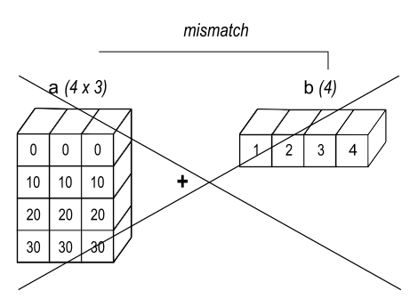
When operating on two arrays, NumPy compares their shapes element-wise. It starts with the trailing (i.e. rightmost) dimension and works its way left. Two dimensions are compatible when - they are equal, or - one of them is 1.
If these conditions are not met, a ValueError: operands could not be broadcast together exception is thrown, indicating that the arrays have incompatible shapes.
Broadcasting is then performed over the missing or length 1 dimensions.
Examples:
A (2d array): 5 x 4
B (1d array): 1
Result (2d array): 5 x 4
A (2d array): 5 x 4
B (1d array): 4
Result (2d array): 5 x 4
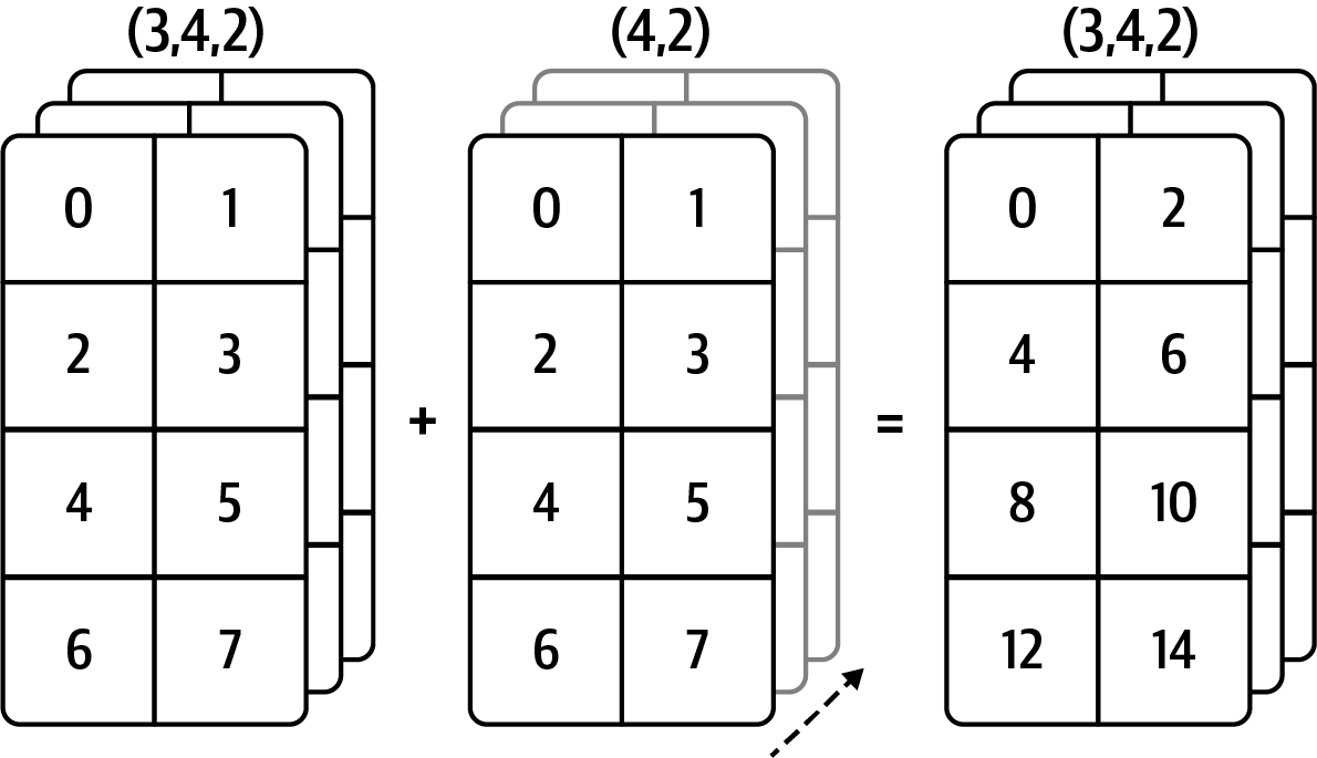
A (3d array): 15 x 3 x 5
B (3d array): 15 x 1 x 5
Result (3d array): 15 x 3 x 5
A (3d array): 15 x 3 x 5
B (2d array): 3 x 5
Result (3d array): 15 x 3 x 5
A (3d array): 15 x 3 x 5
B (2d array): 3 x 1
Result (3d array): 15 x 3 x 5 Broadcasting illustrations
From Python for Data Analysis:
Row
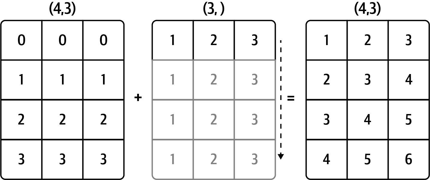
Column
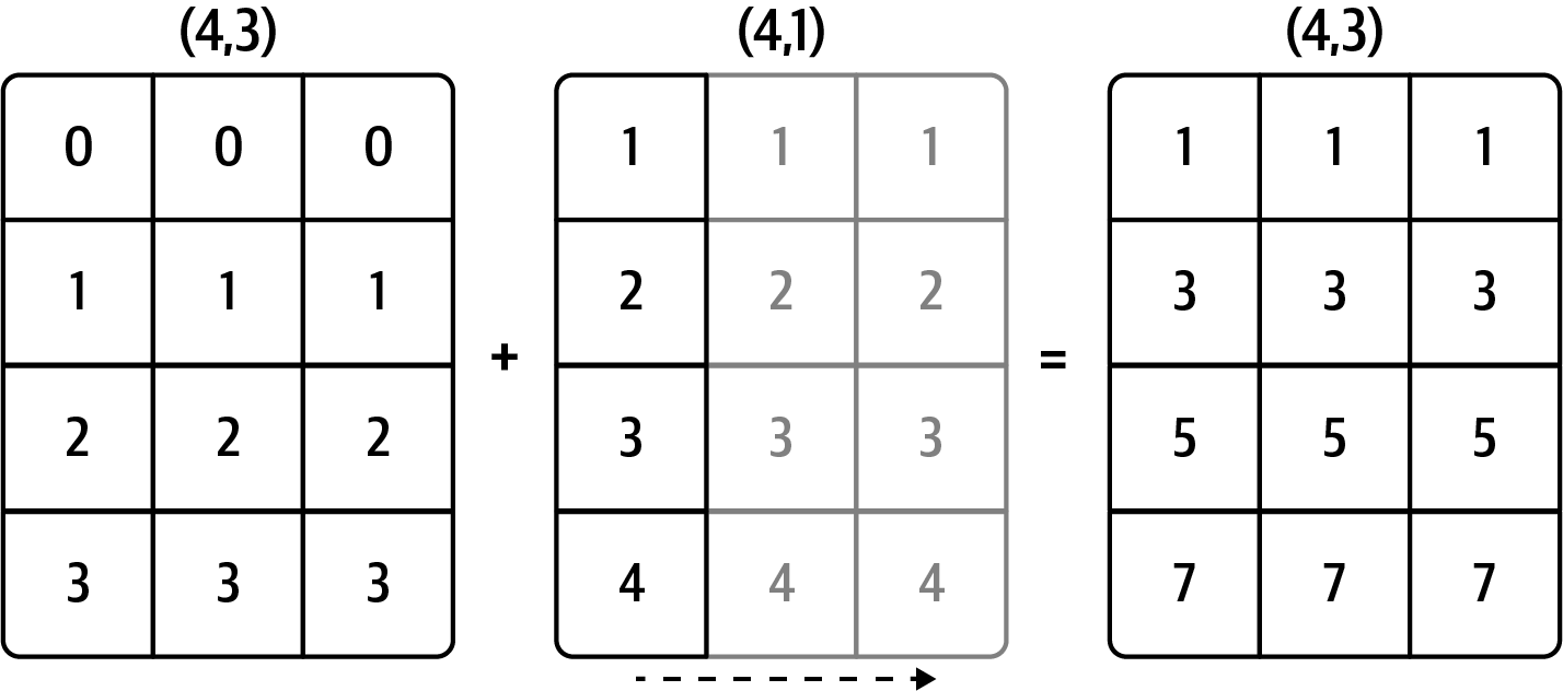
Array
From NumPy docs:
V = np.arange(12).reshape(3, 4)
u3 = np.arange(3)*0.1   # vector size 3
u4 = np.arange(4)*0.01  # vector size 4
V
array([[ 0, 1, 2, 3],
[ 4, 5, 6, 7],
[ 8, 9, 10, 11]])u3array([0. , 0.1, 0.2])# V + u3
# this failsu3.reshape((3, 1))array([[0. ],
[0.1],
[0.2]])V + u3.reshape((3, 1)) # broadcasting u3 horizontally along axis of length 1array([[ 0. , 1. , 2. , 3. ],
[ 4.1, 5.1, 6.1, 7.1],
[ 8.2, 9.2, 10.2, 11.2]])# Same as copying u3 four times:
np.allclose(
V + u3.reshape((3, 1)),
V + np.column_stack([u3, u3, u3, u3]))
# column_stack is short for turning u3 into a (3,1) vector, then hstackTruenp.column_stack([u3, u3, u3, u3])array([[0. , 0. , 0. , 0. ],
[0.1, 0.1, 0.1, 0.1],
[0.2, 0.2, 0.2, 0.2]])np.hstack([u3.reshape(3,1), u3.reshape(3,1), u3.reshape(3,1), u3.reshape(3,1)])array([[0. , 0. , 0. , 0. ],
[0.1, 0.1, 0.1, 0.1],
[0.2, 0.2, 0.2, 0.2]])V * u4.reshape((1, 4)) # broadcasting u4 vertically along axis of length 1array([[0. , 0.01, 0.04, 0.09],
[0. , 0.05, 0.12, 0.21],
[0. , 0.09, 0.2 , 0.33]])V * u4 # this works because trailing dim matchesarray([[0. , 0.01, 0.04, 0.09],
[0. , 0.05, 0.12, 0.21],
[0. , 0.09, 0.2 , 0.33]])# Same as the sum of three u4 stacked vertically:
np.allclose(
V * u4.reshape((1, 4)),
V * np.stack([u4, u4, u4 ]))True# what happens with a 3x3 matrix?
test = np.arange(9).reshape(3,3)
test2 = np.array([1,2,3])
test3 = np.array([6,7,8]).reshape(3,1)test array([[0, 1, 2],
[3, 4, 5],
[6, 7, 8]])test2array([1, 2, 3])test3array([[6],
[7],
[8]])test + test2 # row vectors with shape (1,3) or (3,) will be added to each rowarray([[ 1, 3, 5],
[ 4, 6, 8],
[ 7, 9, 11]])test + test3 # column vectors (3,1) will be added to each columnarray([[ 6, 7, 8],
[10, 11, 12],
[14, 15, 16]])More examples
np.random.normal(size=(4, 4)) * np.random.normal(size=(4, 1))array([[-0.03831005, -0.09974464, -0.48978027, -0.23845806],
[-0.44937391, 1.03127044, 0.33521515, -1.71992523],
[-0.15529269, 0.18452151, 0.32436358, -0.29309952],
[-0.19141432, -0.17290051, 0.15580827, 0.05740805]])A = np.array(range(2*3*4)).reshape((2,3,4))B = A * np.array([1, -1, 2, -2]).reshape((1,1,4))B.shape(2, 3, 4)A[:, :, 1]array([[ 1, 5, 9],
[13, 17, 21]])B[:, :, 1]array([[ -1, -5, -9],
[-13, -17, -21]])More examples
A (2d array)      4 x 1
B (1d array)          3
Result (2d array) 4 x 3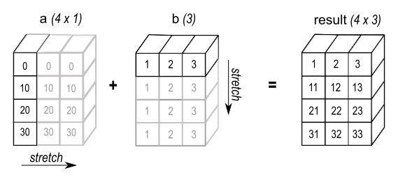
3d array example:
C = np.array(np.arange(5*2)).reshape((5,2))Carray([[0, 1],
[2, 3],
[4, 5],
[6, 7],
[8, 9]])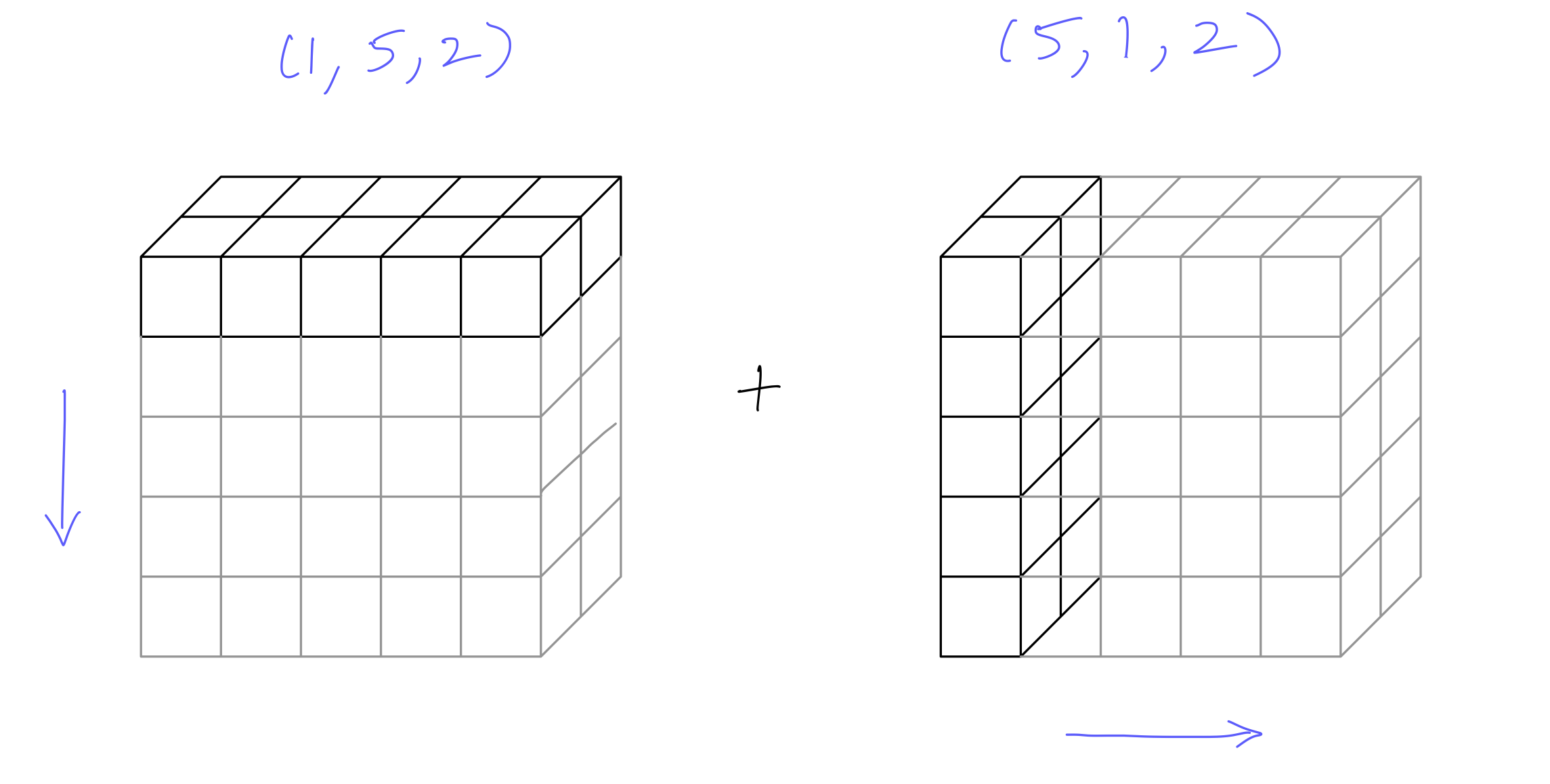
out = C[np.newaxis, :, :] + C[:, np.newaxis, :]C1 1 x 5 x 2
C2 5 x 1 x 2
Result 5 x 5 x 2out.shape(5, 5, 2)out[:, :, 0]array([[ 0, 2, 4, 6, 8],
[ 2, 4, 6, 8, 10],
[ 4, 6, 8, 10, 12],
[ 6, 8, 10, 12, 14],
[ 8, 10, 12, 14, 16]])Multiply many matrices:
S = np.stack([np.random.randn(2, 2) for a in range(5)]).round(2)
S.shape
S
array([[[-1.11, -1.2 ],
[ 0.81, 1.36]],
[[-0.07, 1. ],
[ 0.36, -0.65]],
[[ 0.36, 1.54],
[-0.04, 1.56]],
[[-2.62, 0.82],
[ 0.09, -0.3 ]],
[[ 0.09, -1.99],
[-0.22, 0.36]]])Computing inverses of the five matrices one by one
S[0]

S[0, :, :]

np.linalg.inv(S[0])
array([[-2.5297619 , -2.23214286],
[ 1.50669643, 2.06473214]])With many matrices:
S = np.stack([np.random.randn(2, 2) for a in range(100000)])
S.shape
(100000, 2, 2)from timeit import default_timer as timer
# fast
start = timer()
np.linalg.inv(S)
end = timer()
print(end - start)
# slow
start = timer()
[np.linalg.inv(mat) for mat in S]
end = timer()
print(end - start)0.022097625071182847
0.2965899580158293