from nycflights13 import flights, airports, airlines, planes, weatherLecture 3 - Pandas II
Overview
This lecture introduces:
- the concept of tidy data
- more advanced Pandas functionality, including
groupby, categorical datatypes, hierarchical indexing and merging datasets
References
This lecture contains material from:
- Chapter 8, Python for Data Analysis, 3E (Wes McKinney, 2022)
- Chapter 3, Data Science: A First Introduction with Python (Timbers et al. 2022)
- Pierre Bellec’s notes
- Hadley Wickham. Tidy data. Journal of Statistical Software, 59(10):1–23, 2014.
Tidy Data
Let’s define the following helpful terms:
- variable: a characteristic, number, or quantity that can be measured.
- observation: all of the measurements for a given entity.
- value: a single measurement of a single variable for a given entity.
A tidy data frame satisfies the following three criteria (Wickham, 2014):
- each row is a single observation,
- each column is a single variable, and
- each value is a single cell (i.e., its entry in the data frame is not shared with another value).

Illustration: NYC flights data
We now look at NYC flights data, contained in the nycflights13 packge.
This package contains information about all flights that departed from NYC (e.g. EWR, JFK and LGA) to destinations in the United States, Puerto Rico, and the American Virgin Islands) in 2013: 336,776 flights in total. To help understand what causes delays, it also includes a number of other useful datasets.
This package provides the following data tables.
- flights: all flights that departed from NYC in 2013
- weather: hourly meterological data for each airport
- planes: construction information about each plane
- airports: airport names and locations
- airlines: translation between two letter carrier codes and names
Install the nycflights13 dataset in your conda environment:
'Terminal
conda activate msds597
pip install nycflights13
Load the nycflights13 data:
import numpy as np
import pandas as pd
import seaborn as snsflights.head()| year | month | day | dep_time | sched_dep_time | dep_delay | arr_time | sched_arr_time | arr_delay | carrier | flight | tailnum | origin | dest | air_time | distance | hour | minute | time_hour | |
|---|---|---|---|---|---|---|---|---|---|---|---|---|---|---|---|---|---|---|---|
| 0 | 2013 | 1 | 1 | 517.0 | 515 | 2.0 | 830.0 | 819 | 11.0 | UA | 1545 | N14228 | EWR | IAH | 227.0 | 1400 | 5 | 15 | 2013-01-01T10:00:00Z |
| 1 | 2013 | 1 | 1 | 533.0 | 529 | 4.0 | 850.0 | 830 | 20.0 | UA | 1714 | N24211 | LGA | IAH | 227.0 | 1416 | 5 | 29 | 2013-01-01T10:00:00Z |
| 2 | 2013 | 1 | 1 | 542.0 | 540 | 2.0 | 923.0 | 850 | 33.0 | AA | 1141 | N619AA | JFK | MIA | 160.0 | 1089 | 5 | 40 | 2013-01-01T10:00:00Z |
| 3 | 2013 | 1 | 1 | 544.0 | 545 | -1.0 | 1004.0 | 1022 | -18.0 | B6 | 725 | N804JB | JFK | BQN | 183.0 | 1576 | 5 | 45 | 2013-01-01T10:00:00Z |
| 4 | 2013 | 1 | 1 | 554.0 | 600 | -6.0 | 812.0 | 837 | -25.0 | DL | 461 | N668DN | LGA | ATL | 116.0 | 762 | 6 | 0 | 2013-01-01T11:00:00Z |
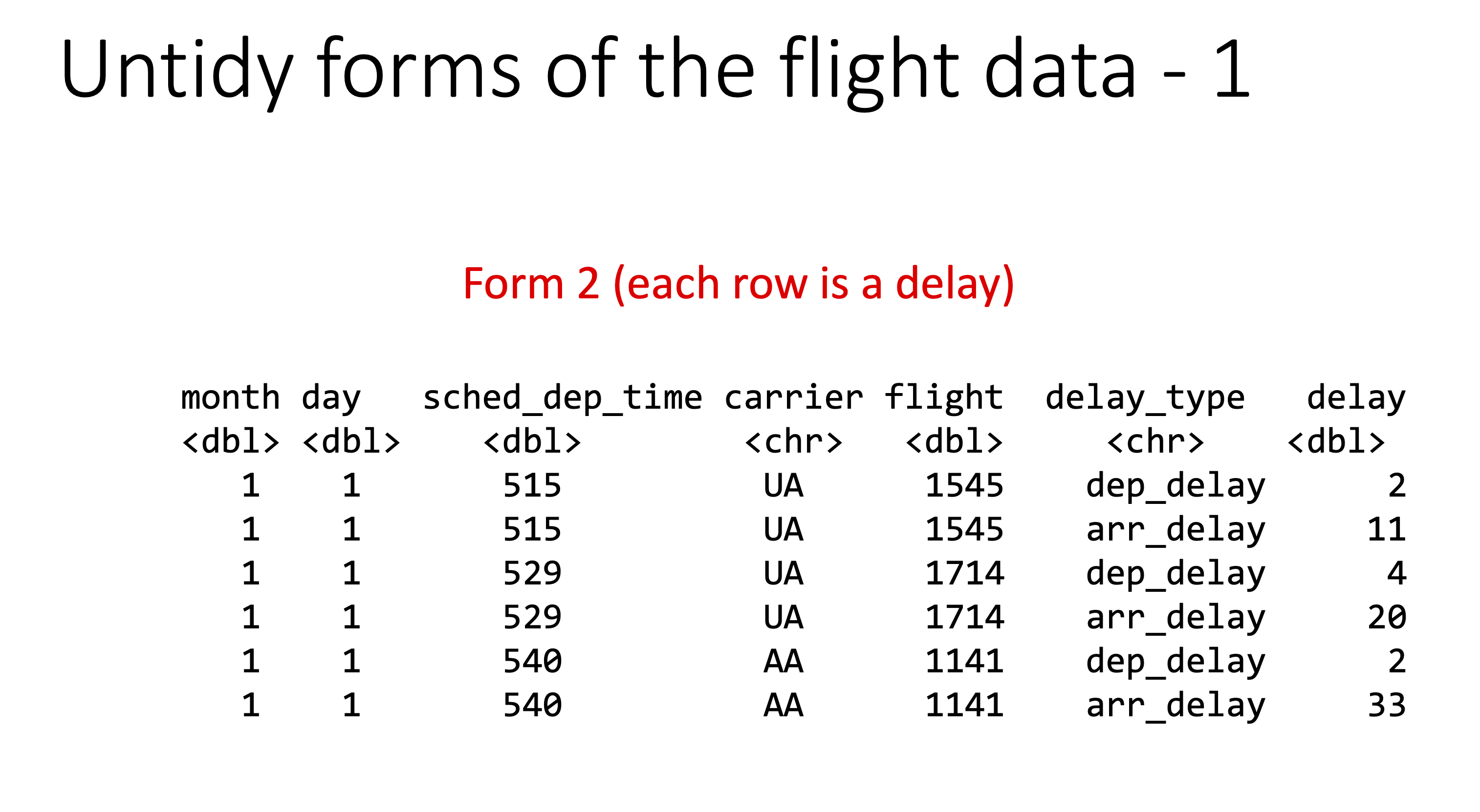
The above data is “tidy”:
- each row is a single observation (flight)
- each column is a single variable (e.g. year, month, departure time)
- each value is a single cell
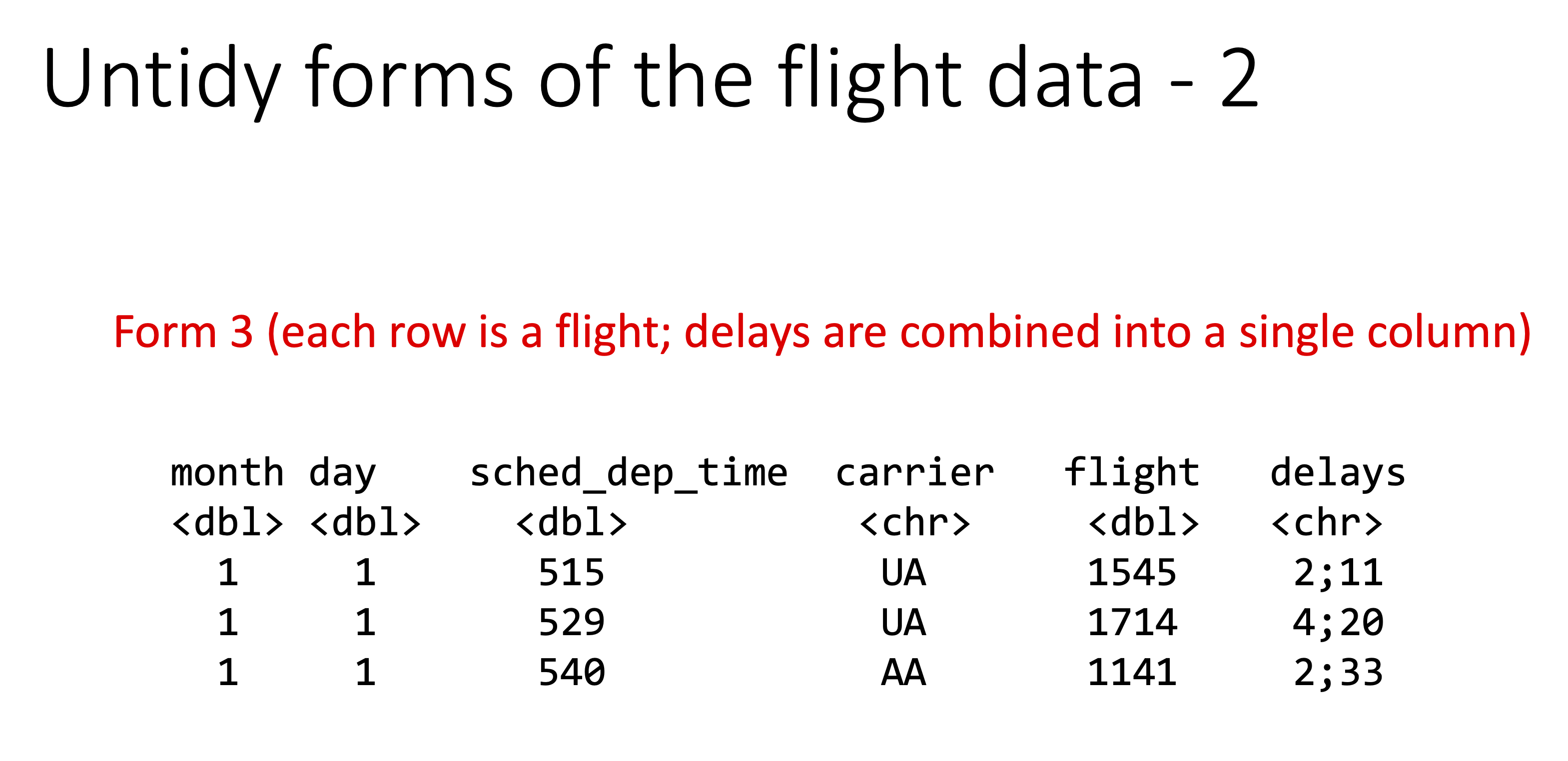
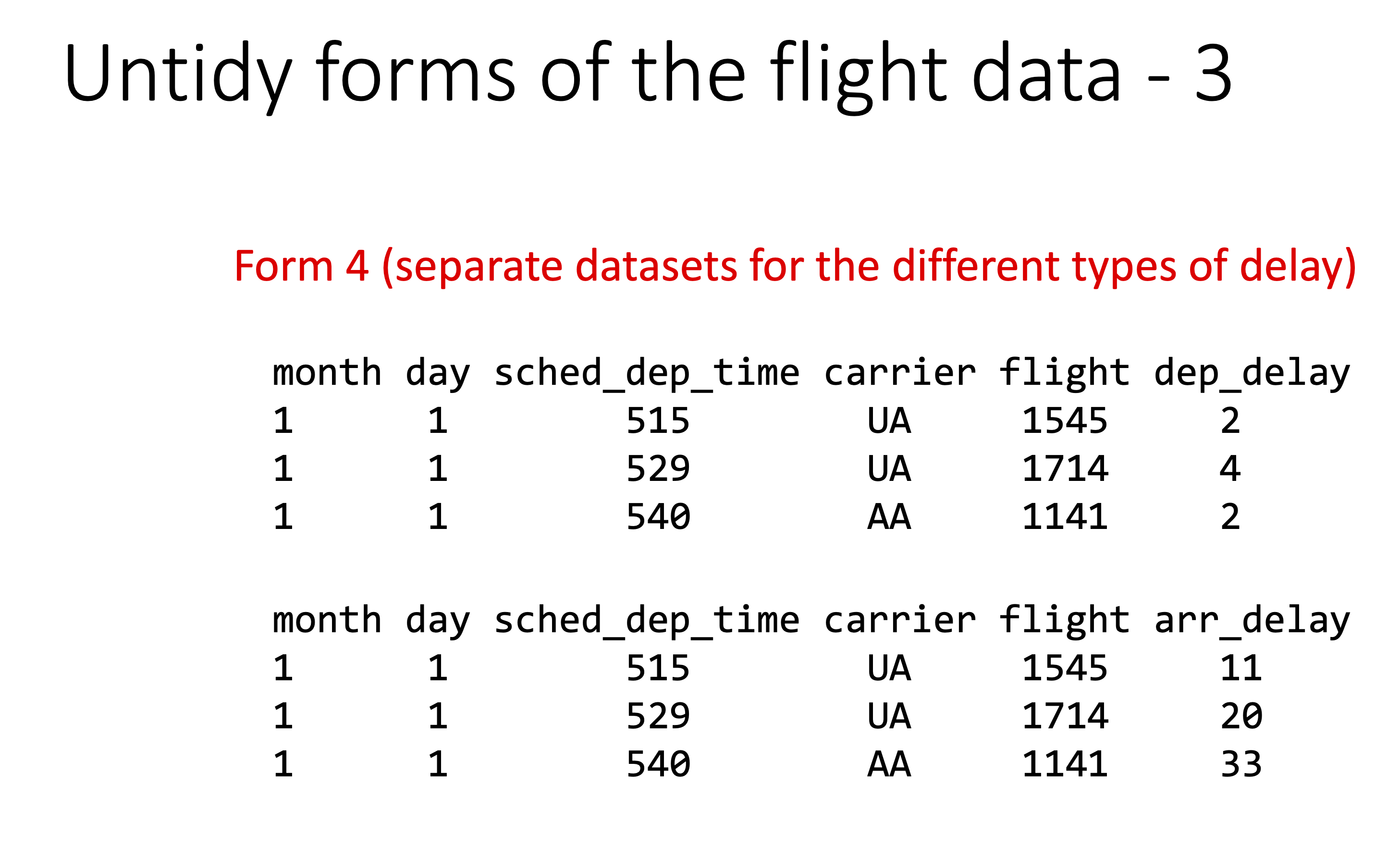
Below are examples of “untidy” versions of this data.
Let’s check the origin of all the flights:
flights['origin'].value_counts()origin
EWR 120835
JFK 111279
LGA 104662
Name: count, dtype: int64Practising skills from last lecture:
- Which flights on 1st Jan have missing departure times?
jan1 = flights[(flights.month == 1) & (flights.day == 1)]jan1[jan1.dep_time.isna()]| year | month | day | dep_time | sched_dep_time | dep_delay | arr_time | sched_arr_time | arr_delay | carrier | flight | tailnum | origin | dest | air_time | distance | hour | minute | time_hour | |
|---|---|---|---|---|---|---|---|---|---|---|---|---|---|---|---|---|---|---|---|
| 838 | 2013 | 1 | 1 | NaN | 1630 | NaN | NaN | 1815 | NaN | EV | 4308 | N18120 | EWR | RDU | NaN | 416 | 16 | 30 | 2013-01-01T21:00:00Z |
| 839 | 2013 | 1 | 1 | NaN | 1935 | NaN | NaN | 2240 | NaN | AA | 791 | N3EHAA | LGA | DFW | NaN | 1389 | 19 | 35 | 2013-01-02T00:00:00Z |
| 840 | 2013 | 1 | 1 | NaN | 1500 | NaN | NaN | 1825 | NaN | AA | 1925 | N3EVAA | LGA | MIA | NaN | 1096 | 15 | 0 | 2013-01-01T20:00:00Z |
| 841 | 2013 | 1 | 1 | NaN | 600 | NaN | NaN | 901 | NaN | B6 | 125 | N618JB | JFK | FLL | NaN | 1069 | 6 | 0 | 2013-01-01T11:00:00Z |
jan1[jan1.dep_time.isna()]['flight']
# we can't do this!
# jan1[jan1.dep_time.isna(), 'flight']

# we CAN do this
jan1.loc[jan1.dep_time.isna(), 'flight']
838 4308
839 791
840 1925
841 125
Name: flight, dtype: int64- Which flights flew to Houston (IAH or HOU)?
houston = flights[(flights.dest == 'IAH') | (flights.dest == 'HOU')]- Which flights that departed from JFK were operated by United, American or Delta? (UA, AA, DL)
jfk = flights[flights.origin == 'JFK']ua = jfk.carrier == 'UA'
aa = jfk.carrier == 'AA'
dl = jfk.carrier == 'DL'
jfk[((ua | aa) | dl)]| year | month | day | dep_time | sched_dep_time | dep_delay | arr_time | sched_arr_time | arr_delay | carrier | flight | tailnum | origin | dest | air_time | distance | hour | minute | time_hour | |
|---|---|---|---|---|---|---|---|---|---|---|---|---|---|---|---|---|---|---|---|
| 2 | 2013 | 1 | 1 | 542.0 | 540 | 2.0 | 923.0 | 850 | 33.0 | AA | 1141 | N619AA | JFK | MIA | 160.0 | 1089 | 5 | 40 | 2013-01-01T10:00:00Z |
| 12 | 2013 | 1 | 1 | 558.0 | 600 | -2.0 | 924.0 | 917 | 7.0 | UA | 194 | N29129 | JFK | LAX | 345.0 | 2475 | 6 | 0 | 2013-01-01T11:00:00Z |
| 23 | 2013 | 1 | 1 | 606.0 | 610 | -4.0 | 837.0 | 845 | -8.0 | DL | 1743 | N3739P | JFK | ATL | 128.0 | 760 | 6 | 10 | 2013-01-01T11:00:00Z |
| 26 | 2013 | 1 | 1 | 611.0 | 600 | 11.0 | 945.0 | 931 | 14.0 | UA | 303 | N532UA | JFK | SFO | 366.0 | 2586 | 6 | 0 | 2013-01-01T11:00:00Z |
| 36 | 2013 | 1 | 1 | 628.0 | 630 | -2.0 | 1137.0 | 1140 | -3.0 | AA | 413 | N3BAAA | JFK | SJU | 192.0 | 1598 | 6 | 30 | 2013-01-01T11:00:00Z |
| ... | ... | ... | ... | ... | ... | ... | ... | ... | ... | ... | ... | ... | ... | ... | ... | ... | ... | ... | ... |
| 336704 | 2013 | 9 | 30 | 2028.0 | 1910 | 78.0 | 2255.0 | 2215 | 40.0 | AA | 21 | N338AA | JFK | LAX | 294.0 | 2475 | 19 | 10 | 2013-09-30T23:00:00Z |
| 336715 | 2013 | 9 | 30 | 2041.0 | 2045 | -4.0 | 2147.0 | 2208 | -21.0 | DL | 985 | N359NB | JFK | BOS | 37.0 | 187 | 20 | 45 | 2013-10-01T00:00:00Z |
| 336718 | 2013 | 9 | 30 | 2050.0 | 2045 | 5.0 | 20.0 | 53 | -33.0 | DL | 347 | N396DA | JFK | SJU | 188.0 | 1598 | 20 | 45 | 2013-10-01T00:00:00Z |
| 336744 | 2013 | 9 | 30 | 2121.0 | 2100 | 21.0 | 2349.0 | 14 | -25.0 | DL | 2363 | N193DN | JFK | LAX | 296.0 | 2475 | 21 | 0 | 2013-10-01T01:00:00Z |
| 336751 | 2013 | 9 | 30 | 2140.0 | 2140 | 0.0 | 10.0 | 40 | -30.0 | AA | 185 | N335AA | JFK | LAX | 298.0 | 2475 | 21 | 40 | 2013-10-01T01:00:00Z |
39018 rows × 19 columns
- Sort the flights to find the most delayed flights.
flights.sort_values(by='arr_delay', ascending=False)| year | month | day | dep_time | sched_dep_time | dep_delay | arr_time | sched_arr_time | arr_delay | carrier | flight | tailnum | origin | dest | air_time | distance | hour | minute | time_hour | |
|---|---|---|---|---|---|---|---|---|---|---|---|---|---|---|---|---|---|---|---|
| 7072 | 2013 | 1 | 9 | 641.0 | 900 | 1301.0 | 1242.0 | 1530 | 1272.0 | HA | 51 | N384HA | JFK | HNL | 640.0 | 4983 | 9 | 0 | 2013-01-09T14:00:00Z |
| 235778 | 2013 | 6 | 15 | 1432.0 | 1935 | 1137.0 | 1607.0 | 2120 | 1127.0 | MQ | 3535 | N504MQ | JFK | CMH | 74.0 | 483 | 19 | 35 | 2013-06-15T23:00:00Z |
| 8239 | 2013 | 1 | 10 | 1121.0 | 1635 | 1126.0 | 1239.0 | 1810 | 1109.0 | MQ | 3695 | N517MQ | EWR | ORD | 111.0 | 719 | 16 | 35 | 2013-01-10T21:00:00Z |
| 327043 | 2013 | 9 | 20 | 1139.0 | 1845 | 1014.0 | 1457.0 | 2210 | 1007.0 | AA | 177 | N338AA | JFK | SFO | 354.0 | 2586 | 18 | 45 | 2013-09-20T22:00:00Z |
| 270376 | 2013 | 7 | 22 | 845.0 | 1600 | 1005.0 | 1044.0 | 1815 | 989.0 | MQ | 3075 | N665MQ | JFK | CVG | 96.0 | 589 | 16 | 0 | 2013-07-22T20:00:00Z |
| ... | ... | ... | ... | ... | ... | ... | ... | ... | ... | ... | ... | ... | ... | ... | ... | ... | ... | ... | ... |
| 336771 | 2013 | 9 | 30 | NaN | 1455 | NaN | NaN | 1634 | NaN | 9E | 3393 | NaN | JFK | DCA | NaN | 213 | 14 | 55 | 2013-09-30T18:00:00Z |
| 336772 | 2013 | 9 | 30 | NaN | 2200 | NaN | NaN | 2312 | NaN | 9E | 3525 | NaN | LGA | SYR | NaN | 198 | 22 | 0 | 2013-10-01T02:00:00Z |
| 336773 | 2013 | 9 | 30 | NaN | 1210 | NaN | NaN | 1330 | NaN | MQ | 3461 | N535MQ | LGA | BNA | NaN | 764 | 12 | 10 | 2013-09-30T16:00:00Z |
| 336774 | 2013 | 9 | 30 | NaN | 1159 | NaN | NaN | 1344 | NaN | MQ | 3572 | N511MQ | LGA | CLE | NaN | 419 | 11 | 59 | 2013-09-30T15:00:00Z |
| 336775 | 2013 | 9 | 30 | NaN | 840 | NaN | NaN | 1020 | NaN | MQ | 3531 | N839MQ | LGA | RDU | NaN | 431 | 8 | 40 | 2013-09-30T12:00:00Z |
336776 rows × 19 columns
- Select columns which have arrival related information.
[col for col in flights.columns if 'arr_' in col]['arr_time', 'sched_arr_time', 'arr_delay']- List the top three airlines that operated flights from EWR the maximum # times and arrange them in descending order.
ewr = flights[flights.origin == 'EWR']ewr.carrier.value_counts().sort_values(ascending=False)carrier
UA 46087
EV 43939
B6 6557
WN 6188
US 4405
DL 4342
AA 3487
MQ 2276
VX 1566
9E 1268
AS 714
OO 6
Name: count, dtype: int64- What are the most common flight routes?
def cat_func(x):
    base = ''
    for i in x:
        base += i + ' '
    return base

origin_dest = flights[['origin', 'dest']].apply(cat_func, axis=1)origin_dest.value_counts(ascending=False)JFK LAX 11262
LGA ATL 10263
LGA ORD 8857
JFK SFO 8204
LGA CLT 6168
...
JFK STL 1
JFK MEM 1
JFK BHM 1
LGA LEX 1
EWR LGA 1
Name: count, Length: 224, dtype: int64- How many flights were there from NYC airports to Seattle (SEA)?
nyc_sea = flights[(flights['origin'].isin(['JFK', 'LGA', 'EWR'])) & (flights['dest'] == 'SEA')]
nyc_sea.shape
(3923, 19)- How many carriers fly to SEA?
len(nyc_sea.carrier.unique()) # or nyc_sea.carrier.nunique()5- What is the average arrival delay?
nyc_sea['arr_delay'].mean()np.float64(-1.0990990990990992)- What proportion of flights come from each NYC airport?
ewr = 100 * (nyc_sea.origin == 'EWR').mean()
lga = 100 * (nyc_sea.origin == 'LGA').mean()
jfk = 100 * (nyc_sea.origin == 'JFK').mean()
f'EWR is {ewr:.2f}%, LGA is {lga:.2f}%, JFK is {jfk:.2f}%''EWR is 46.67%, LGA is 0.00%, JFK is 53.33%'Groupby
In “wide” format, it is easy to apply functions to each of the currencies: e.g. finding the mean of USD, JPY etc. What about in the “tidy” format? Here, we can use the groupby method:
df_wide = pd.read_csv('../data/rates.csv')
df_wide.Time = pd.to_datetime(df_wide.Time)
df_long = df_wide.melt(id_vars='Time', var_name='currency', value_name='rate')df_long.groupby('currency')['rate'].mean()currency
BGN 1.955800
CHF 0.957208
CZK 25.199081
DKK 7.456484
GBP 0.855201
JPY 162.195484
USD 1.082711
Name: rate, dtype: float64df_long.groupby('currency')['rate'].agg(['min', 'max'])| min | max | |
|---|---|---|
| currency | ||
| BGN | 1.95580 | 1.95580 |
| CHF | 0.93150 | 0.98460 |
| CZK | 24.73400 | 25.46000 |
| DKK | 7.45360 | 7.46090 |
| GBP | 0.85098 | 0.85846 |
| JPY | 158.96000 | 164.97000 |
| USD | 1.06370 | 1.09390 |
With groupby, the tidy format is much more consistent than the wide format for many operations. (It is also similar to R’s dplyr and the R tidyverse more generally.)
df_long.groupby('Time')['rate'].agg(['min', 'max'])| min | max | |
|---|---|---|
| Time | ||
| 2024-01-18 | 0.85773 | 160.89 |
| 2024-01-19 | 0.85825 | 161.17 |
| 2024-01-22 | 0.85575 | 160.95 |
| 2024-01-23 | 0.85493 | 160.88 |
| 2024-01-24 | 0.85543 | 160.46 |
| ... | ... | ... |
| 2024-04-10 | 0.85515 | 164.89 |
| 2024-04-11 | 0.85525 | 164.18 |
| 2024-04-12 | 0.85424 | 163.16 |
| 2024-04-15 | 0.85405 | 164.05 |
| 2024-04-16 | 0.85440 | 164.54 |
62 rows × 2 columns
Compare to:
df_wide.agg(['min', 'max'])| Time | USD | JPY | BGN | CZK | DKK | GBP | CHF | |
|---|---|---|---|---|---|---|---|---|
| min | 2024-01-18 | 1.0637 | 158.96 | 1.9558 | 24.734 | 7.4536 | 0.85098 | 0.9315 |
| max | 2024-04-16 | 1.0939 | 164.97 | 1.9558 | 25.460 | 7.4609 | 0.85846 | 0.9846 |
# this fails because we have time as a column
# df_wide.agg(['min', 'max'], axis=1)
# first, get only currency columns (not Time)
cols = df_wide.columns[df_wide.columns != 'Time']
# agg over rows, excluding Time column
df_wide[cols].agg(['min', 'max'], axis=1)| min | max | |
|---|---|---|
| 0 | 0.85440 | 164.54 |
| 1 | 0.85405 | 164.05 |
| 2 | 0.85424 | 163.16 |
| 3 | 0.85525 | 164.18 |
| 4 | 0.85515 | 164.89 |
| ... | ... | ... |
| 57 | 0.85543 | 160.46 |
| 58 | 0.85493 | 160.88 |
| 59 | 0.85575 | 160.95 |
| 60 | 0.85825 | 161.17 |
| 61 | 0.85773 | 160.89 |
62 rows × 2 columns
# alternatively, turn Time into the index
df_wide.index = df_wide.Time
df_wide.drop(columns='Time').agg(['min', 'max'], axis=1)| min | max | |
|---|---|---|
| Time | ||
| 2024-04-16 | 0.85440 | 164.54 |
| 2024-04-15 | 0.85405 | 164.05 |
| 2024-04-12 | 0.85424 | 163.16 |
| 2024-04-11 | 0.85525 | 164.18 |
| 2024-04-10 | 0.85515 | 164.89 |
| ... | ... | ... |
| 2024-01-24 | 0.85543 | 160.46 |
| 2024-01-23 | 0.85493 | 160.88 |
| 2024-01-22 | 0.85575 | 160.95 |
| 2024-01-19 | 0.85825 | 161.17 |
| 2024-01-18 | 0.85773 | 160.89 |
62 rows × 2 columns
Back to nycflights13: - Which airline carrier had the longest mean delay?
flights.groupby('carrier')['arr_delay'].mean().sort_values(ascending=False)carrier
F9 21.920705
FL 20.115906
EV 15.796431
YV 15.556985
OO 11.931034
MQ 10.774733
WN 9.649120
B6 9.457973
9E 7.379669
UA 3.558011
US 2.129595
VX 1.764464
DL 1.644341
AA 0.364291
HA -6.915205
AS -9.930889
Name: arr_delay, dtype: float64- What days of week had highest mean delay times?
# convert time hour to datetime dtype
flights['time_hour'] = pd.to_datetime(flights['time_hour'])

# You can get day of week as integer (Monday=0, Sunday=6)
flights['dayofweek'] = flights['time_hour'].dt.dayofweek

# You can also get day name:
flights['day_name'] = flights['time_hour'].dt.day_name()flights.groupby('day_name')['arr_delay'].mean().sort_values(ascending=False)day_name
Thursday 11.044998
Monday 9.846577
Friday 9.397136
Wednesday 6.581860
Tuesday 6.118452
Sunday 2.645165
Saturday 1.126204
Name: arr_delay, dtype: float64- What month had highest mean delay times?
flights.groupby('month')['arr_delay'].mean().sort_values(ascending=False)month
7 16.711307
6 16.481330
12 14.870355
4 11.176063
1 6.129972
8 6.040652
3 5.807577
2 5.613019
5 3.521509
11 0.461347
10 -0.167063
9 -4.018364
Name: arr_delay, dtype: float64- What day-of-week / month combo had largest mean delay times?
flights.groupby(['month', 'day_name'])['arr_delay'].mean().sort_values(ascending=False)month day_name
6 Monday 30.650388
7 Monday 29.503160
4 Friday 25.632658
Thursday 24.991816
8 Thursday 22.258595
...
5 Tuesday -4.991189
9 Tuesday -6.252610
Wednesday -7.006858
Sunday -8.932241
Saturday -12.576506
Name: arr_delay, Length: 84, dtype: float64- What unique day had the largest mean delay times?
flights.groupby(['month', 'day'])['arr_delay'].mean().sort_values(ascending=False)month day
3 8 85.862155
6 13 63.753689
7 22 62.763403
5 23 61.970899
7 10 59.626478
...
9 5 -15.540373
28 -16.371852
6 -17.895010
10 1 -18.959375
9 7 -20.349854
Name: arr_delay, Length: 365, dtype: float64- Plot the delays by month for each carrier:
sns.relplot(data=flights,
            x='month',
            y='arr_delay',
            hue='carrier',
            kind='line') # default in relplot is a scatterplot - we want a line plot here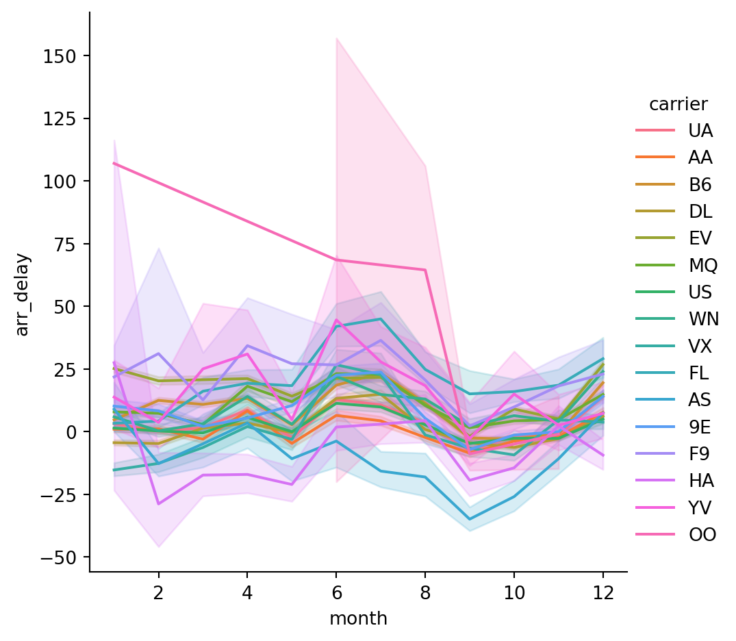
The default behavior in seaborn is to aggregate the multiple measurements at each x value by plotting the mean and the 95% confidence interval around the mean, where the confidence interval is calculated using bootstrapping.
sns.relplot(data=flights,
            x='month',
            y='arr_delay',
            hue='carrier',
            kind='line',
            errorbar=None) # can disable with errorbar = None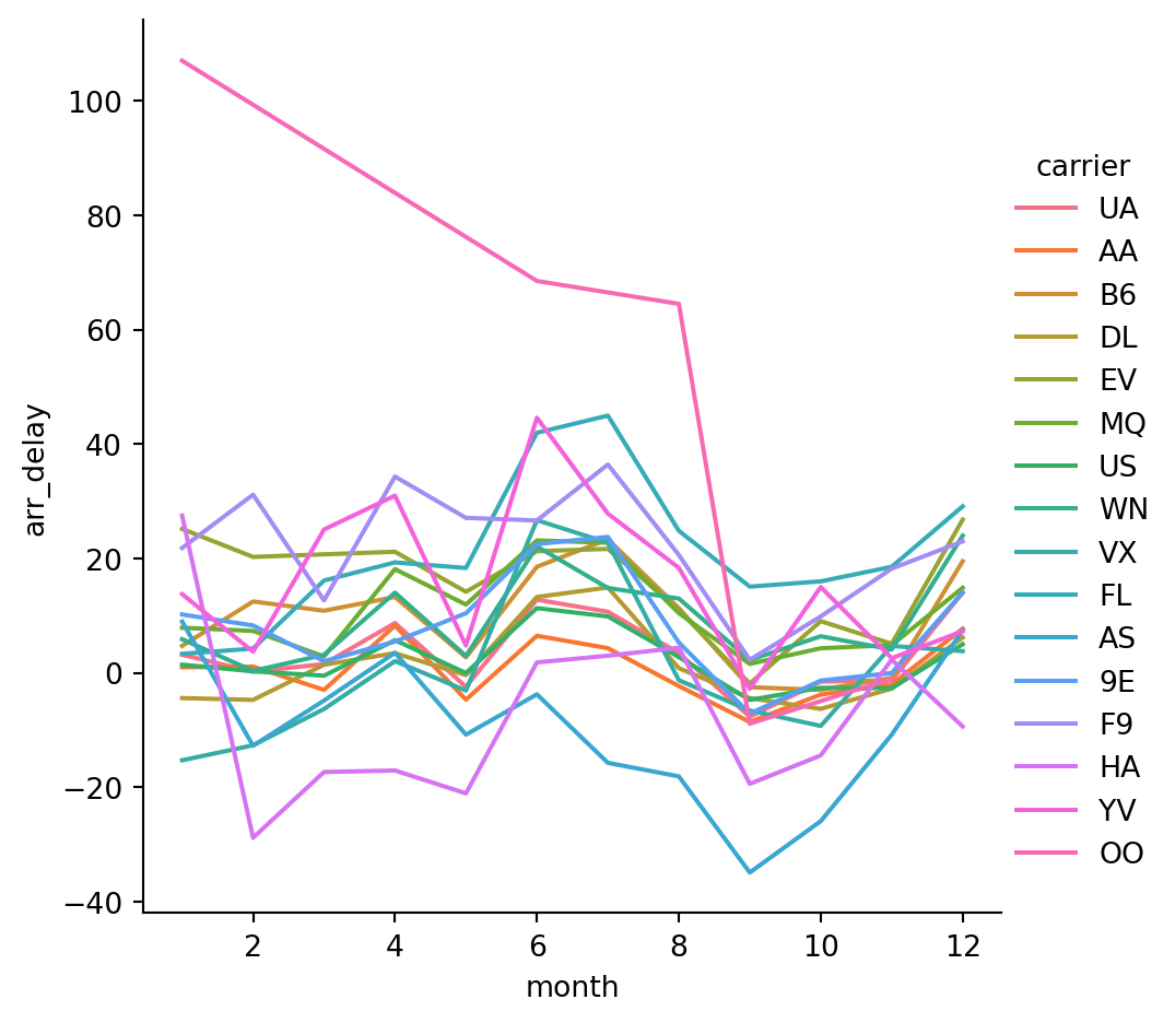
- Now only plot the top 5 carriers (by number of flights)
top_carriers = flights['carrier'].value_counts().reset_index()
top_carriers = top_carriers.carrier[0:5]
top_carriers = top_carriers.to_list()flights_subset = flights[flights.carrier.isin(top_carriers)]sns.relplot(data=flights_subset,
x='month',
y='arr_delay',
hue='carrier',
kind='line',
height = 4,
aspect = 3)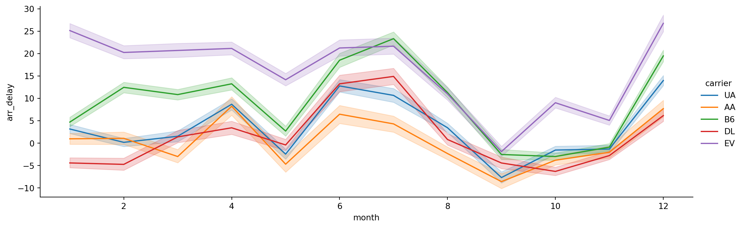
- What about by hour of day?
sns.relplot(data=flights_subset,
            x='hour',
            y='arr_delay',
            hue='carrier',
            kind='line',
            height = 4,
            aspect = 3)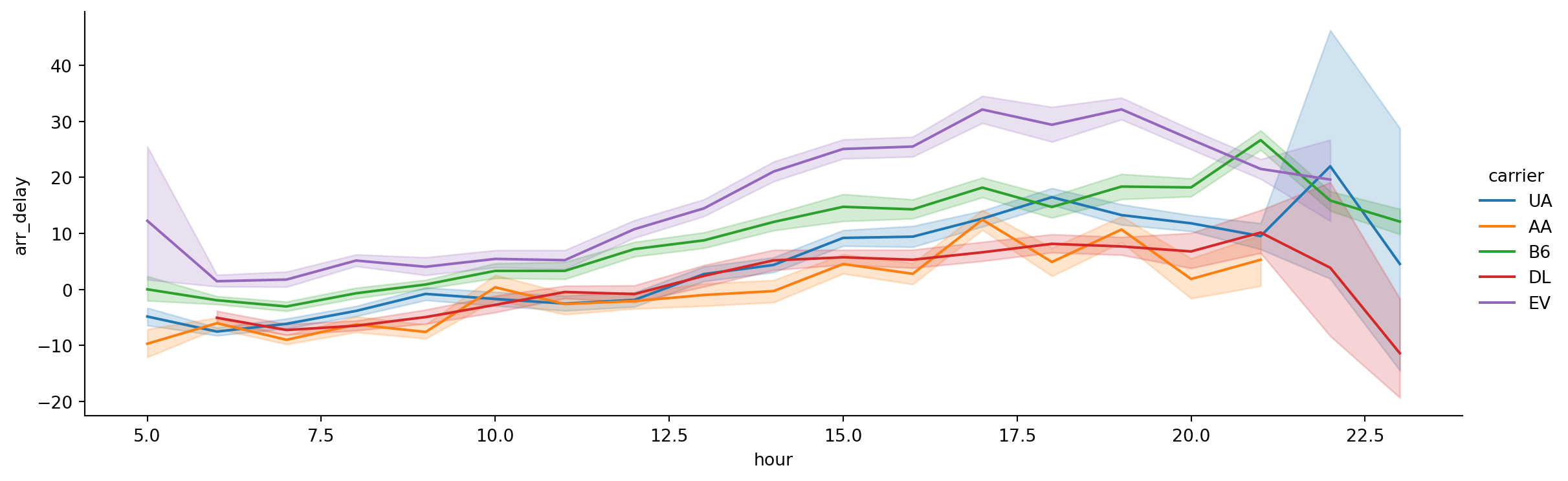
Categorical Data
Sometimes you see categorical data (e.g. USD, JPY etc.) represented as integers, often for ease of data storage. These data will also have a look-up table, so you can tell what integer corresponds to what category.
values = pd.Series([0, 1, 0, 0] * 2)
dim = pd.Series(['orange', 'apple'])print(values)0 0
1 1
2 0
3 0
4 0
5 1
6 0
7 0
dtype: int64print(dim)0 orange
1 apple
dtype: objectdim.take(values)0 orange
1 apple
0 orange
0 orange
0 orange
1 apple
0 orange
0 orange
dtype: objectpandas has a special Categorical extension type for holding data that uses the integer-based categorical representation or encoding. This is a popular data compression technique for data with many occurrences of similar values and can provide significantly faster performance with lower memory use, especially for string data.
fruit = pd.Categorical.from_codes(values, dim)fruit['orange', 'apple', 'orange', 'orange', 'orange', 'apple', 'orange', 'orange']
Categories (2, object): ['orange', 'apple']df_long['currency']0 USD
1 USD
2 USD
3 USD
4 USD
...
429 CHF
430 CHF
431 CHF
432 CHF
433 CHF
Name: currency, Length: 434, dtype: objectcurrency_object = df_long['currency'].copy()df_long['currency'] = df_long['currency'].astype('category')df_long['currency']0 USD
1 USD
2 USD
3 USD
4 USD
...
429 CHF
430 CHF
431 CHF
432 CHF
433 CHF
Name: currency, Length: 434, dtype: category
Categories (7, object): ['BGN', 'CHF', 'CZK', 'DKK', 'GBP', 'JPY', 'USD']currency_cat = df_long['currency']currency_object.memory_usage(deep=True)22700currency_cat.memory_usage(deep=True)1230Binning
Continuous data is often discretized or otherwise separated into “bins” for analysis.
For NYC flights data, let’s turn the integer day of week into ‘weekday’ or ‘weekend’ using pd.cut.
pd.cut(flights['dayofweek'], bins=[0, 5, 7], right=False) # right=False specifies do not include right value0 [0, 5)
1 [0, 5)
2 [0, 5)
3 [0, 5)
4 [0, 5)
...
336771 [0, 5)
336772 [0, 5)
336773 [0, 5)
336774 [0, 5)
336775 [0, 5)
Name: dayofweek, Length: 336776, dtype: category
Categories (2, interval[int64, left]): [[0, 5) < [5, 7)]day_type = pd.cut(flights['dayofweek'], bins=[0, 5, 7], labels=['weekday', 'weekend'], right=False) # right=False specifies do not include right valueday_type0 weekday
1 weekday
2 weekday
3 weekday
4 weekday
...
336771 weekday
336772 weekday
336773 weekday
336774 weekday
336775 weekday
Name: dayofweek, Length: 336776, dtype: category
Categories (2, object): ['weekday' < 'weekend']day_type.cat.categoriesIndex(['weekday', 'weekend'], dtype='object')Note that pd.cut produces ordered categories (['weekday' < 'weekend']).
day_type.cat.orderedTrueYou can create a new unordered categorical vector by:
day_type.cat.as_unordered()0 weekday
1 weekday
2 weekday
3 weekday
4 weekday
...
336771 weekday
336772 weekday
336773 weekday
336774 weekday
336775 weekday
Name: dayofweek, Length: 336776, dtype: category
Categories (2, object): ['weekday', 'weekend']Illustration: Penguins data
Missing data
df_penguins = sns.load_dataset('penguins')
df_penguins| species | island | bill_length_mm | bill_depth_mm | flipper_length_mm | body_mass_g | sex | |
|---|---|---|---|---|---|---|---|
| 0 | Adelie | Torgersen | 39.1 | 18.7 | 181.0 | 3750.0 | Male |
| 1 | Adelie | Torgersen | 39.5 | 17.4 | 186.0 | 3800.0 | Female |
| 2 | Adelie | Torgersen | 40.3 | 18.0 | 195.0 | 3250.0 | Female |
| 3 | Adelie | Torgersen | NaN | NaN | NaN | NaN | NaN |
| 4 | Adelie | Torgersen | 36.7 | 19.3 | 193.0 | 3450.0 | Female |
| ... | ... | ... | ... | ... | ... | ... | ... |
| 339 | Gentoo | Biscoe | NaN | NaN | NaN | NaN | NaN |
| 340 | Gentoo | Biscoe | 46.8 | 14.3 | 215.0 | 4850.0 | Female |
| 341 | Gentoo | Biscoe | 50.4 | 15.7 | 222.0 | 5750.0 | Male |
| 342 | Gentoo | Biscoe | 45.2 | 14.8 | 212.0 | 5200.0 | Female |
| 343 | Gentoo | Biscoe | 49.9 | 16.1 | 213.0 | 5400.0 | Male |
344 rows × 7 columns
How to get rid of NaNs?
keep = df_penguins.apply(lambda x: not any(x.isna()), axis=1)df_penguins[keep]| species | island | bill_length_mm | bill_depth_mm | flipper_length_mm | body_mass_g | sex | |
|---|---|---|---|---|---|---|---|
| 0 | Adelie | Torgersen | 39.1 | 18.7 | 181.0 | 3750.0 | Male |
| 1 | Adelie | Torgersen | 39.5 | 17.4 | 186.0 | 3800.0 | Female |
| 2 | Adelie | Torgersen | 40.3 | 18.0 | 195.0 | 3250.0 | Female |
| 4 | Adelie | Torgersen | 36.7 | 19.3 | 193.0 | 3450.0 | Female |
| 5 | Adelie | Torgersen | 39.3 | 20.6 | 190.0 | 3650.0 | Male |
| ... | ... | ... | ... | ... | ... | ... | ... |
| 338 | Gentoo | Biscoe | 47.2 | 13.7 | 214.0 | 4925.0 | Female |
| 340 | Gentoo | Biscoe | 46.8 | 14.3 | 215.0 | 4850.0 | Female |
| 341 | Gentoo | Biscoe | 50.4 | 15.7 | 222.0 | 5750.0 | Male |
| 342 | Gentoo | Biscoe | 45.2 | 14.8 | 212.0 | 5200.0 | Female |
| 343 | Gentoo | Biscoe | 49.9 | 16.1 | 213.0 | 5400.0 | Male |
333 rows × 7 columns
Alternatively, use the dropna method:
df_penguins.dropna() # drop rows with at least one NaN| species | island | bill_length_mm | bill_depth_mm | flipper_length_mm | body_mass_g | sex | |
|---|---|---|---|---|---|---|---|
| 0 | Adelie | Torgersen | 39.1 | 18.7 | 181.0 | 3750.0 | Male |
| 1 | Adelie | Torgersen | 39.5 | 17.4 | 186.0 | 3800.0 | Female |
| 2 | Adelie | Torgersen | 40.3 | 18.0 | 195.0 | 3250.0 | Female |
| 4 | Adelie | Torgersen | 36.7 | 19.3 | 193.0 | 3450.0 | Female |
| 5 | Adelie | Torgersen | 39.3 | 20.6 | 190.0 | 3650.0 | Male |
| ... | ... | ... | ... | ... | ... | ... | ... |
| 338 | Gentoo | Biscoe | 47.2 | 13.7 | 214.0 | 4925.0 | Female |
| 340 | Gentoo | Biscoe | 46.8 | 14.3 | 215.0 | 4850.0 | Female |
| 341 | Gentoo | Biscoe | 50.4 | 15.7 | 222.0 | 5750.0 | Male |
| 342 | Gentoo | Biscoe | 45.2 | 14.8 | 212.0 | 5200.0 | Female |
| 343 | Gentoo | Biscoe | 49.9 | 16.1 | 213.0 | 5400.0 | Male |
333 rows × 7 columns
We can also fill the NaNs with a particular value if we have some prior knowledge of what the values should be:
df_penguins.fillna(0)| species | island | bill_length_mm | bill_depth_mm | flipper_length_mm | body_mass_g | sex | |
|---|---|---|---|---|---|---|---|
| 0 | Adelie | Torgersen | 39.1 | 18.7 | 181.0 | 3750.0 | Male |
| 1 | Adelie | Torgersen | 39.5 | 17.4 | 186.0 | 3800.0 | Female |
| 2 | Adelie | Torgersen | 40.3 | 18.0 | 195.0 | 3250.0 | Female |
| 3 | Adelie | Torgersen | 0.0 | 0.0 | 0.0 | 0.0 | 0 |
| 4 | Adelie | Torgersen | 36.7 | 19.3 | 193.0 | 3450.0 | Female |
| ... | ... | ... | ... | ... | ... | ... | ... |
| 339 | Gentoo | Biscoe | 0.0 | 0.0 | 0.0 | 0.0 | 0 |
| 340 | Gentoo | Biscoe | 46.8 | 14.3 | 215.0 | 4850.0 | Female |
| 341 | Gentoo | Biscoe | 50.4 | 15.7 | 222.0 | 5750.0 | Male |
| 342 | Gentoo | Biscoe | 45.2 | 14.8 | 212.0 | 5200.0 | Female |
| 343 | Gentoo | Biscoe | 49.9 | 16.1 | 213.0 | 5400.0 | Male |
344 rows × 7 columns
We can fill the values with different values for different columns:
df_penguins.fillna({'bill_length_mm': 0, 'sex': 'Female'})| species | island | bill_length_mm | bill_depth_mm | flipper_length_mm | body_mass_g | sex | |
|---|---|---|---|---|---|---|---|
| 0 | Adelie | Torgersen | 39.1 | 18.7 | 181.0 | 3750.0 | Male |
| 1 | Adelie | Torgersen | 39.5 | 17.4 | 186.0 | 3800.0 | Female |
| 2 | Adelie | Torgersen | 40.3 | 18.0 | 195.0 | 3250.0 | Female |
| 3 | Adelie | Torgersen | 0.0 | NaN | NaN | NaN | Female |
| 4 | Adelie | Torgersen | 36.7 | 19.3 | 193.0 | 3450.0 | Female |
| ... | ... | ... | ... | ... | ... | ... | ... |
| 339 | Gentoo | Biscoe | 0.0 | NaN | NaN | NaN | Female |
| 340 | Gentoo | Biscoe | 46.8 | 14.3 | 215.0 | 4850.0 | Female |
| 341 | Gentoo | Biscoe | 50.4 | 15.7 | 222.0 | 5750.0 | Male |
| 342 | Gentoo | Biscoe | 45.2 | 14.8 | 212.0 | 5200.0 | Female |
| 343 | Gentoo | Biscoe | 49.9 | 16.1 | 213.0 | 5400.0 | Male |
344 rows × 7 columns
df_penguins.mean(numeric_only=True)bill_length_mm 43.921930
bill_depth_mm 17.151170
flipper_length_mm 200.915205
body_mass_g 4201.754386
dtype: float64We can fill in with other values, like the mean:
df_penguins.fillna(df_penguins.mean(numeric_only=True))| species | island | bill_length_mm | bill_depth_mm | flipper_length_mm | body_mass_g | sex | |
|---|---|---|---|---|---|---|---|
| 0 | Adelie | Torgersen | 39.10000 | 18.70000 | 181.000000 | 3750.000000 | Male |
| 1 | Adelie | Torgersen | 39.50000 | 17.40000 | 186.000000 | 3800.000000 | Female |
| 2 | Adelie | Torgersen | 40.30000 | 18.00000 | 195.000000 | 3250.000000 | Female |
| 3 | Adelie | Torgersen | 43.92193 | 17.15117 | 200.915205 | 4201.754386 | NaN |
| 4 | Adelie | Torgersen | 36.70000 | 19.30000 | 193.000000 | 3450.000000 | Female |
| ... | ... | ... | ... | ... | ... | ... | ... |
| 339 | Gentoo | Biscoe | 43.92193 | 17.15117 | 200.915205 | 4201.754386 | NaN |
| 340 | Gentoo | Biscoe | 46.80000 | 14.30000 | 215.000000 | 4850.000000 | Female |
| 341 | Gentoo | Biscoe | 50.40000 | 15.70000 | 222.000000 | 5750.000000 | Male |
| 342 | Gentoo | Biscoe | 45.20000 | 14.80000 | 212.000000 | 5200.000000 | Female |
| 343 | Gentoo | Biscoe | 49.90000 | 16.10000 | 213.000000 | 5400.000000 | Male |
344 rows × 7 columns
For now, let’s proceed with dropping the rows which have an NaN value:
df_penguins = df_penguins.dropna()Checking for duplicated rows
df_penguins.duplicated()0 False
1 False
2 False
4 False
5 False
...
338 False
340 False
341 False
342 False
343 False
Length: 333, dtype: boolany(df_penguins.duplicated())False# if we did have duplicates, we could use
df_penguins.drop_duplicates()| species | island | bill_length_mm | bill_depth_mm | flipper_length_mm | body_mass_g | sex | |
|---|---|---|---|---|---|---|---|
| 0 | Adelie | Torgersen | 39.1 | 18.7 | 181.0 | 3750.0 | Male |
| 1 | Adelie | Torgersen | 39.5 | 17.4 | 186.0 | 3800.0 | Female |
| 2 | Adelie | Torgersen | 40.3 | 18.0 | 195.0 | 3250.0 | Female |
| 4 | Adelie | Torgersen | 36.7 | 19.3 | 193.0 | 3450.0 | Female |
| 5 | Adelie | Torgersen | 39.3 | 20.6 | 190.0 | 3650.0 | Male |
| ... | ... | ... | ... | ... | ... | ... | ... |
| 338 | Gentoo | Biscoe | 47.2 | 13.7 | 214.0 | 4925.0 | Female |
| 340 | Gentoo | Biscoe | 46.8 | 14.3 | 215.0 | 4850.0 | Female |
| 341 | Gentoo | Biscoe | 50.4 | 15.7 | 222.0 | 5750.0 | Male |
| 342 | Gentoo | Biscoe | 45.2 | 14.8 | 212.0 | 5200.0 | Female |
| 343 | Gentoo | Biscoe | 49.9 | 16.1 | 213.0 | 5400.0 | Male |
333 rows × 7 columns
Computing Indicator/Dummy Variables
Another type of transformation for statistical modeling or machine learning applications is converting a categorical variable into a dummy or indicator matrix. If a column in a DataFrame has k distinct values, you would derive a matrix or DataFrame with k columns containing all 1s and 0s. pandas has a pandas.get_dummies function for doing this, though you could also devise one yourself.
pd.get_dummies(df_penguins.sex)| Female | Male | |
|---|---|---|
| 0 | False | True |
| 1 | True | False |
| 2 | True | False |
| 4 | True | False |
| 5 | False | True |
| ... | ... | ... |
| 338 | True | False |
| 340 | True | False |
| 341 | False | True |
| 342 | True | False |
| 343 | False | True |
333 rows × 2 columns
pd.get_dummies(df_penguins.sex, dtype=float)| Female | Male | |
|---|---|---|
| 0 | 0.0 | 1.0 |
| 1 | 1.0 | 0.0 |
| 2 | 1.0 | 0.0 |
| 4 | 1.0 | 0.0 |
| 5 | 0.0 | 1.0 |
| ... | ... | ... |
| 338 | 1.0 | 0.0 |
| 340 | 1.0 | 0.0 |
| 341 | 0.0 | 1.0 |
| 342 | 1.0 | 0.0 |
| 343 | 0.0 | 1.0 |
333 rows × 2 columns
Seaborn pairplot
The default relplot is a scatterplot:
sns.relplot(data=df_penguins,
            x='bill_length_mm',
            y='bill_depth_mm')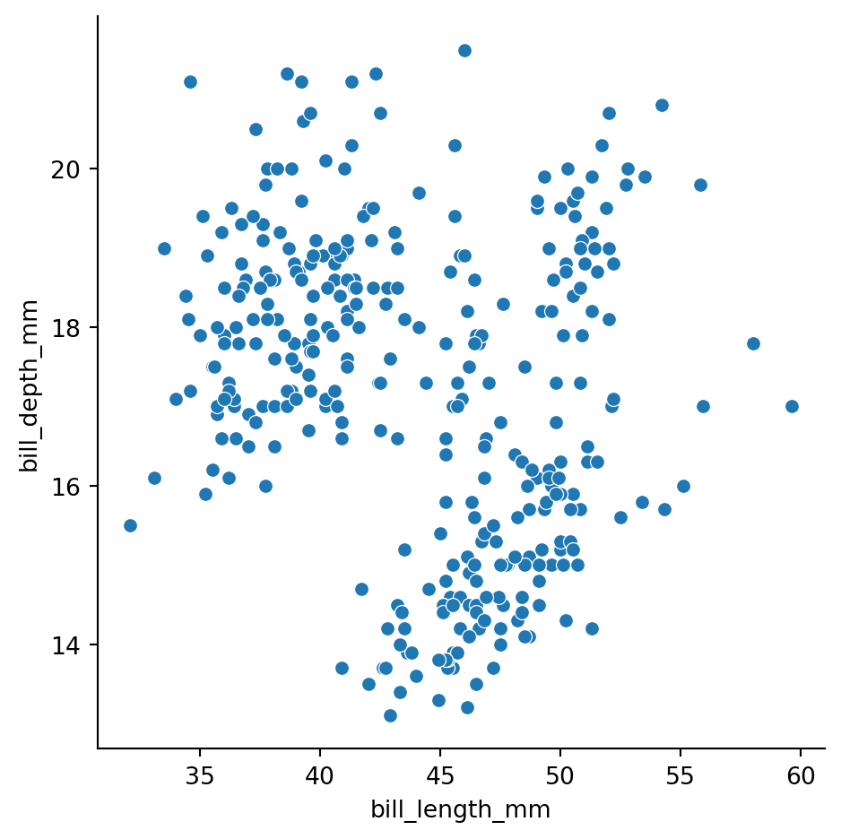
sns.relplot(data=df_penguins,
            x='bill_length_mm',
            y='bill_depth_mm',
            hue='species')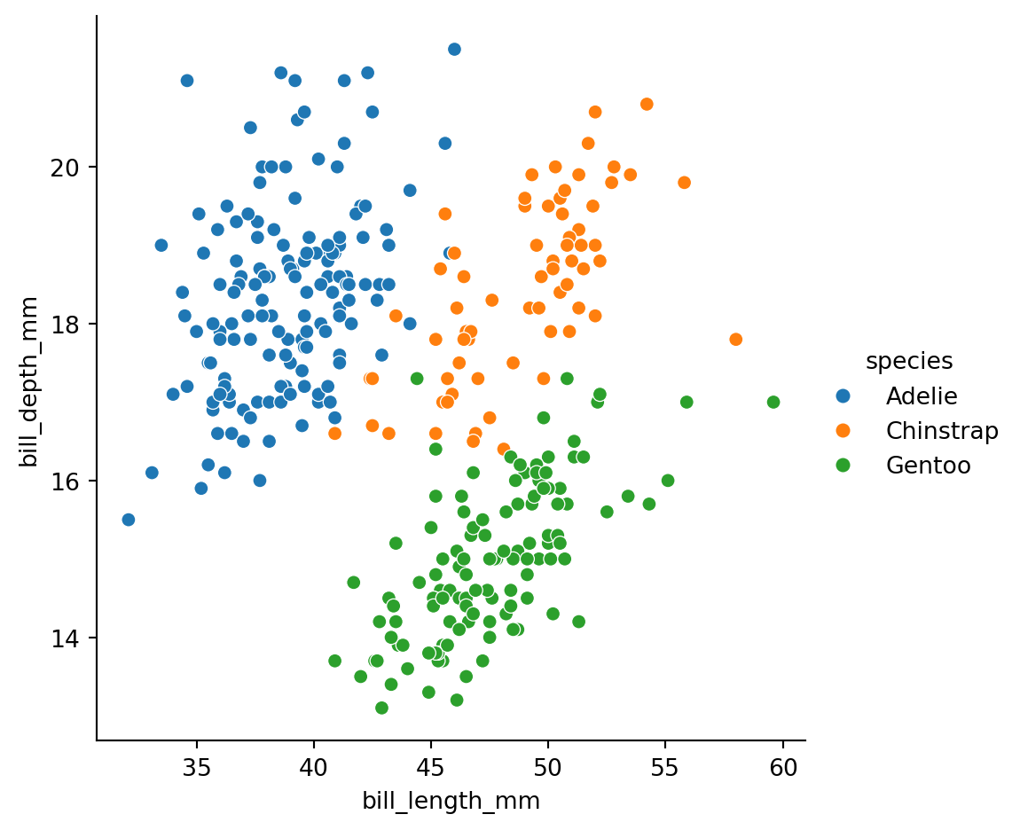
sns.relplot(data=df_penguins,
            x='bill_length_mm',
            y='bill_depth_mm',
            hue='species',
            style='sex')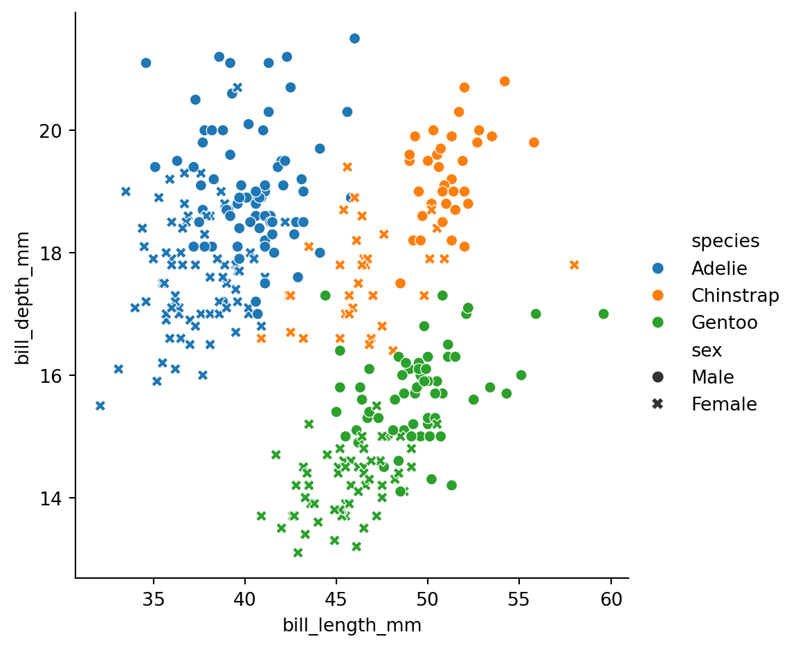
sns.relplot(data=df_penguins,
            x='bill_length_mm',
            y='flipper_length_mm',
            hue='species',
            style='sex')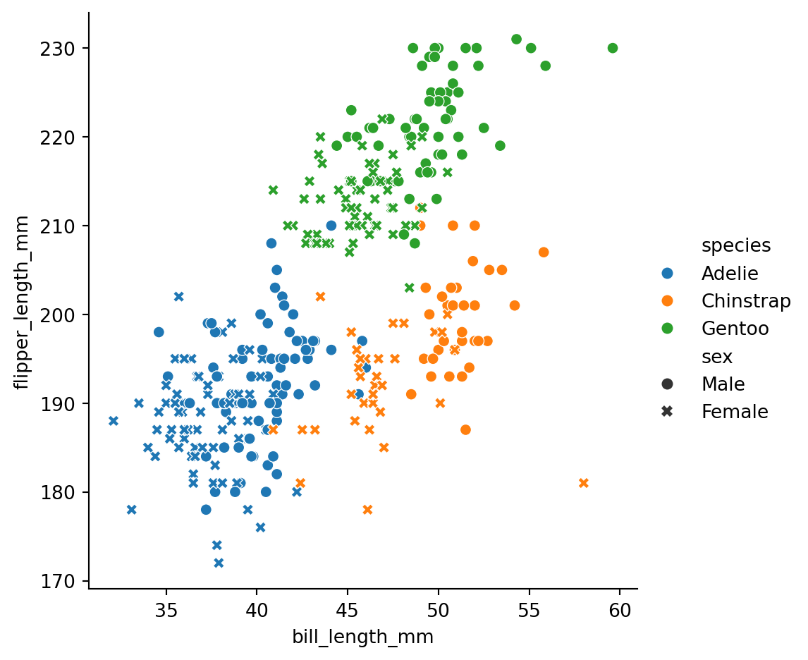
sns.relplot(data=df_penguins,
            x='bill_length_mm',
            y='flipper_length_mm',
            hue='species',
            col='sex')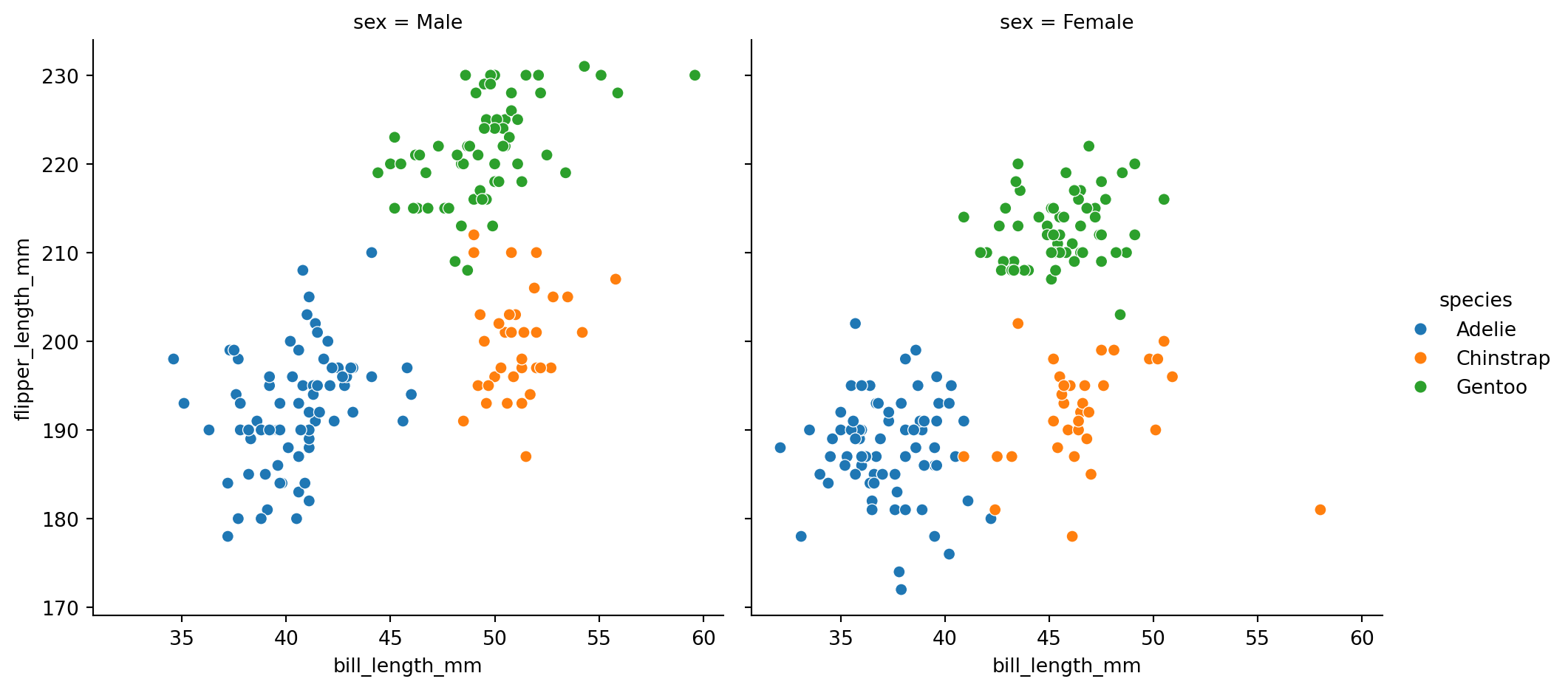
By default, this function will create a grid of Axes such that each numeric variable in data will by shared across the y-axes across a single row and the x-axes across a single column.
sns.pairplot(data=df_penguins, hue='species')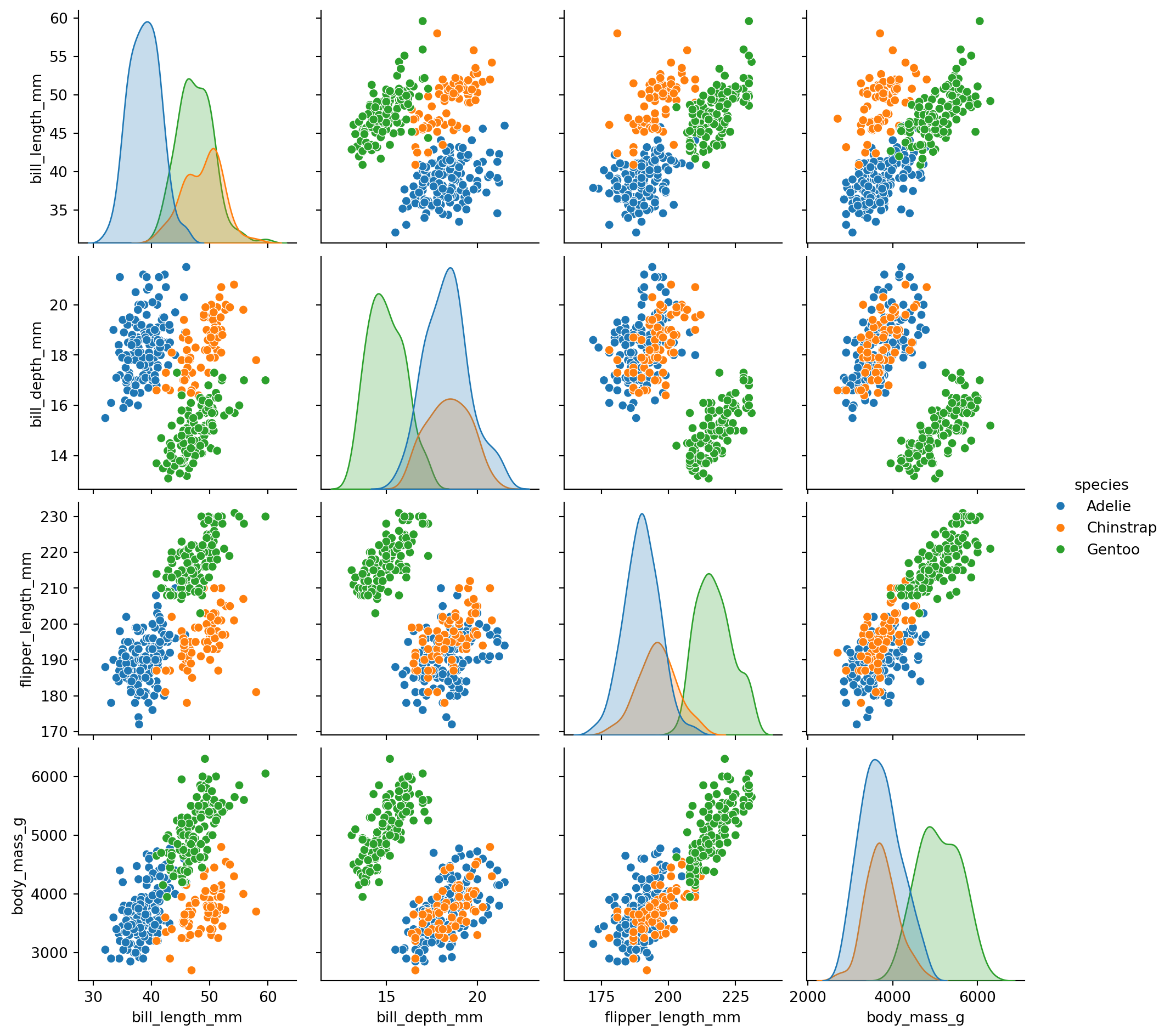
Groupby with multiple categories
Let’s take a look at summary statistics.
With .agg, we can apply several functions at once.
grouped = df_penguins.groupby(['species', 'island', 'sex'])
grouped.agg(['mean', 'median'])| bill_length_mm | bill_depth_mm | flipper_length_mm | body_mass_g | |||||||
|---|---|---|---|---|---|---|---|---|---|---|
| mean | median | mean | median | mean | median | mean | median | |||
| species | island | sex | ||||||||
| Adelie | Biscoe | Female | 37.359091 | 37.75 | 17.704545 | 17.70 | 187.181818 | 187.0 | 3369.318182 | 3375.0 |
| Male | 40.590909 | 40.80 | 19.036364 | 18.90 | 190.409091 | 191.0 | 4050.000000 | 4000.0 | ||
| Dream | Female | 36.911111 | 36.80 | 17.618519 | 17.80 | 187.851852 | 188.0 | 3344.444444 | 3400.0 | |
| Male | 40.071429 | 40.25 | 18.839286 | 18.65 | 191.928571 | 190.5 | 4045.535714 | 3987.5 | ||
| Torgersen | Female | 37.554167 | 37.60 | 17.550000 | 17.45 | 188.291667 | 189.0 | 3395.833333 | 3400.0 | |
| Male | 40.586957 | 41.10 | 19.391304 | 19.20 | 194.913043 | 195.0 | 4034.782609 | 4000.0 | ||
| Chinstrap | Dream | Female | 46.573529 | 46.30 | 17.588235 | 17.65 | 191.735294 | 192.0 | 3527.205882 | 3550.0 |
| Male | 51.094118 | 50.95 | 19.252941 | 19.30 | 199.911765 | 200.5 | 3938.970588 | 3950.0 | ||
| Gentoo | Biscoe | Female | 45.563793 | 45.50 | 14.237931 | 14.25 | 212.706897 | 212.0 | 4679.741379 | 4700.0 |
| Male | 49.473770 | 49.50 | 15.718033 | 15.70 | 221.540984 | 221.0 | 5484.836066 | 5500.0 | ||
Note: .agg with a single function is equivalent to .apply
all(grouped.agg('mean') == grouped.apply('mean'))TrueHierarchical indexing
Hierarchical indexing is an important feature of pandas that enables you to have multiple (two or more) index levels on an axis.
grouped_mm = grouped.agg(['mean', 'median'])grouped_mm.indexMultiIndex([( 'Adelie', 'Biscoe', 'Female'),
( 'Adelie', 'Biscoe', 'Male'),
( 'Adelie', 'Dream', 'Female'),
( 'Adelie', 'Dream', 'Male'),
( 'Adelie', 'Torgersen', 'Female'),
( 'Adelie', 'Torgersen', 'Male'),
('Chinstrap', 'Dream', 'Female'),
('Chinstrap', 'Dream', 'Male'),
( 'Gentoo', 'Biscoe', 'Female'),
( 'Gentoo', 'Biscoe', 'Male')],
names=['species', 'island', 'sex'])Here, the columns also have a MultiIndex.
grouped_mm.columnsMultiIndex([( 'bill_length_mm', 'mean'),
( 'bill_length_mm', 'median'),
( 'bill_depth_mm', 'mean'),
( 'bill_depth_mm', 'median'),
('flipper_length_mm', 'mean'),
('flipper_length_mm', 'median'),
( 'body_mass_g', 'mean'),
( 'body_mass_g', 'median')],
)You can see how many levels an index has by accessing its nlevels attribute:
grouped_mm.index.nlevels3grouped_mm.index.levelsFrozenList([['Adelie', 'Chinstrap', 'Gentoo'], ['Biscoe', 'Dream', 'Torgersen'], ['Female', 'Male']])grouped_mm.columns.nlevels2With partial column indexing you can select groups of columns:
grouped_mm['bill_depth_mm']| mean | median | |||
|---|---|---|---|---|
| species | island | sex | ||
| Adelie | Biscoe | Female | 17.704545 | 17.70 |
| Male | 19.036364 | 18.90 | ||
| Dream | Female | 17.618519 | 17.80 | |
| Male | 18.839286 | 18.65 | ||
| Torgersen | Female | 17.550000 | 17.45 | |
| Male | 19.391304 | 19.20 | ||
| Chinstrap | Dream | Female | 17.588235 | 17.65 |
| Male | 19.252941 | 19.30 | ||
| Gentoo | Biscoe | Female | 14.237931 | 14.25 |
| Male | 15.718033 | 15.70 |
grouped_mm.loc['Adelie']| bill_length_mm | bill_depth_mm | flipper_length_mm | body_mass_g | ||||||
|---|---|---|---|---|---|---|---|---|---|
| mean | median | mean | median | mean | median | mean | median | ||
| island | sex | ||||||||
| Biscoe | Female | 37.359091 | 37.75 | 17.704545 | 17.70 | 187.181818 | 187.0 | 3369.318182 | 3375.0 |
| Male | 40.590909 | 40.80 | 19.036364 | 18.90 | 190.409091 | 191.0 | 4050.000000 | 4000.0 | |
| Dream | Female | 36.911111 | 36.80 | 17.618519 | 17.80 | 187.851852 | 188.0 | 3344.444444 | 3400.0 |
| Male | 40.071429 | 40.25 | 18.839286 | 18.65 | 191.928571 | 190.5 | 4045.535714 | 3987.5 | |
| Torgersen | Female | 37.554167 | 37.60 | 17.550000 | 17.45 | 188.291667 | 189.0 | 3395.833333 | 3400.0 |
| Male | 40.586957 | 41.10 | 19.391304 | 19.20 | 194.913043 | 195.0 | 4034.782609 | 4000.0 | |
grouped_mm.loc['Adelie', "body_mass_g"] # works for the level 0 index on the rows or the columns| mean | median | ||
|---|---|---|---|
| island | sex | ||
| Biscoe | Female | 3369.318182 | 3375.0 |
| Male | 4050.000000 | 4000.0 | |
| Dream | Female | 3344.444444 | 3400.0 |
| Male | 4045.535714 | 3987.5 | |
| Torgersen | Female | 3395.833333 | 3400.0 |
| Male | 4034.782609 | 4000.0 |
# we can't do this for "inner level"
# grouped_m.loc['Biscoe']
# grouped_mm.loc['Adelie', "mean"]
To traverse levels (i.e. get one key from first level and another key from second level), use tuples:
grouped_mm.loc[('Adelie', 'Biscoe')]| bill_length_mm | bill_depth_mm | flipper_length_mm | body_mass_g | |||||
|---|---|---|---|---|---|---|---|---|
| mean | median | mean | median | mean | median | mean | median | |
| sex | ||||||||
| Female | 37.359091 | 37.75 | 17.704545 | 17.7 | 187.181818 | 187.0 | 3369.318182 | 3375.0 |
| Male | 40.590909 | 40.80 | 19.036364 | 18.9 | 190.409091 | 191.0 | 4050.000000 | 4000.0 |
grouped_mm.loc[('Adelie', 'Biscoe'), ('bill_length_mm', 'mean')]sex
Female 37.359091
Male 40.590909
Name: (bill_length_mm, mean), dtype: float64grouped_mm.loc[:, ('bill_length_mm', 'mean')]species island sex
Adelie Biscoe Female 37.359091
Male 40.590909
Dream Female 36.911111
Male 40.071429
Torgersen Female 37.554167
Male 40.586957
Chinstrap Dream Female 46.573529
Male 51.094118
Gentoo Biscoe Female 45.563793
Male 49.473770
Name: (bill_length_mm, mean), dtype: float64A list is used to specify multiple keys:
grouped_mm.loc[['Adelie', 'Gentoo'], ["body_mass_g", "flipper_length_mm"]]| body_mass_g | flipper_length_mm | |||||
|---|---|---|---|---|---|---|
| mean | median | mean | median | |||
| species | island | sex | ||||
| Adelie | Biscoe | Female | 3369.318182 | 3375.0 | 187.181818 | 187.0 |
| Male | 4050.000000 | 4000.0 | 190.409091 | 191.0 | ||
| Dream | Female | 3344.444444 | 3400.0 | 187.851852 | 188.0 | |
| Male | 4045.535714 | 3987.5 | 191.928571 | 190.5 | ||
| Torgersen | Female | 3395.833333 | 3400.0 | 188.291667 | 189.0 | |
| Male | 4034.782609 | 4000.0 | 194.913043 | 195.0 | ||
| Gentoo | Biscoe | Female | 4679.741379 | 4700.0 | 212.706897 | 212.0 |
| Male | 5484.836066 | 5500.0 | 221.540984 | 221.0 | ||
# list of tuples
grouped_mm.loc[[('Adelie', 'Dream', 'Male'), ('Gentoo', 'Biscoe', 'Female')]]| bill_length_mm | bill_depth_mm | flipper_length_mm | body_mass_g | |||||||
|---|---|---|---|---|---|---|---|---|---|---|
| mean | median | mean | median | mean | median | mean | median | |||
| species | island | sex | ||||||||
| Adelie | Dream | Male | 40.071429 | 40.25 | 18.839286 | 18.65 | 191.928571 | 190.5 | 4045.535714 | 3987.5 |
| Gentoo | Biscoe | Female | 45.563793 | 45.50 | 14.237931 | 14.25 | 212.706897 | 212.0 | 4679.741379 | 4700.0 |
It is important to note that tuples and lists are not treated identically in pandas when it comes to indexing. Whereas a tuple is interpreted as one multi-level key, a list is used to specify several keys. Or in other words, tuples go horizontally (traversing levels), lists go vertically (scanning levels).
See more examples here: https://pandas.pydata.org/docs/user_guide/advanced.html#advanced-indexing-with-hierarchical-index
s = pd.Series(
    [1, 2, 3, 4, 5, 6],
    index=pd.MultiIndex.from_product([["A", "B"], ["c", "d", "e"]]),
)
s
A c 1
d 2
e 3
B c 4
d 5
e 6
dtype: int64s.loc[[("A", "c"), ("B", "d")]] # list of tuplesA c 1
B d 5
dtype: int64s.loc[(["A", "B"], ["c", "d"])] # tuple of listsA c 1
d 2
B c 4
d 5
dtype: int64Reordering and sorting levels
At times you may need to rearrange the order of the levels on an axis or sort the data by the values in one specific level. The swaplevel method takes two level numbers or names and returns a new object with the levels interchanged (but the data is otherwise unaltered):
grouped_mm.swaplevel('species', 'island')| bill_length_mm | bill_depth_mm | flipper_length_mm | body_mass_g | |||||||
|---|---|---|---|---|---|---|---|---|---|---|
| mean | median | mean | median | mean | median | mean | median | |||
| island | species | sex | ||||||||
| Biscoe | Adelie | Female | 37.359091 | 37.75 | 17.704545 | 17.70 | 187.181818 | 187.0 | 3369.318182 | 3375.0 |
| Male | 40.590909 | 40.80 | 19.036364 | 18.90 | 190.409091 | 191.0 | 4050.000000 | 4000.0 | ||
| Dream | Adelie | Female | 36.911111 | 36.80 | 17.618519 | 17.80 | 187.851852 | 188.0 | 3344.444444 | 3400.0 |
| Male | 40.071429 | 40.25 | 18.839286 | 18.65 | 191.928571 | 190.5 | 4045.535714 | 3987.5 | ||
| Torgersen | Adelie | Female | 37.554167 | 37.60 | 17.550000 | 17.45 | 188.291667 | 189.0 | 3395.833333 | 3400.0 |
| Male | 40.586957 | 41.10 | 19.391304 | 19.20 | 194.913043 | 195.0 | 4034.782609 | 4000.0 | ||
| Dream | Chinstrap | Female | 46.573529 | 46.30 | 17.588235 | 17.65 | 191.735294 | 192.0 | 3527.205882 | 3550.0 |
| Male | 51.094118 | 50.95 | 19.252941 | 19.30 | 199.911765 | 200.5 | 3938.970588 | 3950.0 | ||
| Biscoe | Gentoo | Female | 45.563793 | 45.50 | 14.237931 | 14.25 | 212.706897 | 212.0 | 4679.741379 | 4700.0 |
| Male | 49.473770 | 49.50 | 15.718033 | 15.70 | 221.540984 | 221.0 | 5484.836066 | 5500.0 | ||
grouped_mm.swaplevel('species', 'island').sort_index()| bill_length_mm | bill_depth_mm | flipper_length_mm | body_mass_g | |||||||
|---|---|---|---|---|---|---|---|---|---|---|
| mean | median | mean | median | mean | median | mean | median | |||
| island | species | sex | ||||||||
| Biscoe | Adelie | Female | 37.359091 | 37.75 | 17.704545 | 17.70 | 187.181818 | 187.0 | 3369.318182 | 3375.0 |
| Male | 40.590909 | 40.80 | 19.036364 | 18.90 | 190.409091 | 191.0 | 4050.000000 | 4000.0 | ||
| Gentoo | Female | 45.563793 | 45.50 | 14.237931 | 14.25 | 212.706897 | 212.0 | 4679.741379 | 4700.0 | |
| Male | 49.473770 | 49.50 | 15.718033 | 15.70 | 221.540984 | 221.0 | 5484.836066 | 5500.0 | ||
| Dream | Adelie | Female | 36.911111 | 36.80 | 17.618519 | 17.80 | 187.851852 | 188.0 | 3344.444444 | 3400.0 |
| Male | 40.071429 | 40.25 | 18.839286 | 18.65 | 191.928571 | 190.5 | 4045.535714 | 3987.5 | ||
| Chinstrap | Female | 46.573529 | 46.30 | 17.588235 | 17.65 | 191.735294 | 192.0 | 3527.205882 | 3550.0 | |
| Male | 51.094118 | 50.95 | 19.252941 | 19.30 | 199.911765 | 200.5 | 3938.970588 | 3950.0 | ||
| Torgersen | Adelie | Female | 37.554167 | 37.60 | 17.550000 | 17.45 | 188.291667 | 189.0 | 3395.833333 | 3400.0 |
| Male | 40.586957 | 41.10 | 19.391304 | 19.20 | 194.913043 | 195.0 | 4034.782609 | 4000.0 | ||
grouped_mm.reorder_levels([2, 1, 0], axis=0)| bill_length_mm | bill_depth_mm | flipper_length_mm | body_mass_g | |||||||
|---|---|---|---|---|---|---|---|---|---|---|
| mean | median | mean | median | mean | median | mean | median | |||
| sex | island | species | ||||||||
| Female | Biscoe | Adelie | 37.359091 | 37.75 | 17.704545 | 17.70 | 187.181818 | 187.0 | 3369.318182 | 3375.0 |
| Male | Biscoe | Adelie | 40.590909 | 40.80 | 19.036364 | 18.90 | 190.409091 | 191.0 | 4050.000000 | 4000.0 |
| Female | Dream | Adelie | 36.911111 | 36.80 | 17.618519 | 17.80 | 187.851852 | 188.0 | 3344.444444 | 3400.0 |
| Male | Dream | Adelie | 40.071429 | 40.25 | 18.839286 | 18.65 | 191.928571 | 190.5 | 4045.535714 | 3987.5 |
| Female | Torgersen | Adelie | 37.554167 | 37.60 | 17.550000 | 17.45 | 188.291667 | 189.0 | 3395.833333 | 3400.0 |
| Male | Torgersen | Adelie | 40.586957 | 41.10 | 19.391304 | 19.20 | 194.913043 | 195.0 | 4034.782609 | 4000.0 |
| Female | Dream | Chinstrap | 46.573529 | 46.30 | 17.588235 | 17.65 | 191.735294 | 192.0 | 3527.205882 | 3550.0 |
| Male | Dream | Chinstrap | 51.094118 | 50.95 | 19.252941 | 19.30 | 199.911765 | 200.5 | 3938.970588 | 3950.0 |
| Female | Biscoe | Gentoo | 45.563793 | 45.50 | 14.237931 | 14.25 | 212.706897 | 212.0 | 4679.741379 | 4700.0 |
| Male | Biscoe | Gentoo | 49.473770 | 49.50 | 15.718033 | 15.70 | 221.540984 | 221.0 | 5484.836066 | 5500.0 |
grouped_mm.reorder_levels([1, 0], axis=1)| mean | median | mean | median | mean | median | mean | median | |||
|---|---|---|---|---|---|---|---|---|---|---|
| bill_length_mm | bill_length_mm | bill_depth_mm | bill_depth_mm | flipper_length_mm | flipper_length_mm | body_mass_g | body_mass_g | |||
| species | island | sex | ||||||||
| Adelie | Biscoe | Female | 37.359091 | 37.75 | 17.704545 | 17.70 | 187.181818 | 187.0 | 3369.318182 | 3375.0 |
| Male | 40.590909 | 40.80 | 19.036364 | 18.90 | 190.409091 | 191.0 | 4050.000000 | 4000.0 | ||
| Dream | Female | 36.911111 | 36.80 | 17.618519 | 17.80 | 187.851852 | 188.0 | 3344.444444 | 3400.0 | |
| Male | 40.071429 | 40.25 | 18.839286 | 18.65 | 191.928571 | 190.5 | 4045.535714 | 3987.5 | ||
| Torgersen | Female | 37.554167 | 37.60 | 17.550000 | 17.45 | 188.291667 | 189.0 | 3395.833333 | 3400.0 | |
| Male | 40.586957 | 41.10 | 19.391304 | 19.20 | 194.913043 | 195.0 | 4034.782609 | 4000.0 | ||
| Chinstrap | Dream | Female | 46.573529 | 46.30 | 17.588235 | 17.65 | 191.735294 | 192.0 | 3527.205882 | 3550.0 |
| Male | 51.094118 | 50.95 | 19.252941 | 19.30 | 199.911765 | 200.5 | 3938.970588 | 3950.0 | ||
| Gentoo | Biscoe | Female | 45.563793 | 45.50 | 14.237931 | 14.25 | 212.706897 | 212.0 | 4679.741379 | 4700.0 |
| Male | 49.473770 | 49.50 | 15.718033 | 15.70 | 221.540984 | 221.0 | 5484.836066 | 5500.0 |
Summary statistics by level
Many descriptive and summary statistics on DataFrame and Series have a level option in which you can specify the level you want to aggregate by on a particular axis.
grouped_mm.groupby(level=0).mean()| bill_length_mm | bill_depth_mm | flipper_length_mm | body_mass_g | |||||
|---|---|---|---|---|---|---|---|---|
| mean | median | mean | median | mean | median | mean | median | |
| species | ||||||||
| Adelie | 38.845610 | 39.050 | 18.356670 | 18.283333 | 190.096007 | 190.083333 | 3706.652380 | 3693.75 |
| Chinstrap | 48.833824 | 48.625 | 18.420588 | 18.475000 | 195.823529 | 196.250000 | 3733.088235 | 3750.00 |
| Gentoo | 47.518782 | 47.500 | 14.977982 | 14.975000 | 217.123940 | 216.500000 | 5082.288722 | 5100.00 |
grouped_mm.groupby(level=0, axis='columns').mean() # takes mean over column level=1/var/folders/f0/m7l23y8s7p3_0x04b3td9nyjr2hyc8/T/ipykernel_4760/3198538097.py:1: FutureWarning:
DataFrame.groupby with axis=1 is deprecated. Do `frame.T.groupby(...)` without axis instead.
| bill_depth_mm | bill_length_mm | body_mass_g | flipper_length_mm | |||
|---|---|---|---|---|---|---|
| species | island | sex | ||||
| Adelie | Biscoe | Female | 17.702273 | 37.554545 | 3372.159091 | 187.090909 |
| Male | 18.968182 | 40.695455 | 4025.000000 | 190.704545 | ||
| Dream | Female | 17.709259 | 36.855556 | 3372.222222 | 187.925926 | |
| Male | 18.744643 | 40.160714 | 4016.517857 | 191.214286 | ||
| Torgersen | Female | 17.500000 | 37.577083 | 3397.916667 | 188.645833 | |
| Male | 19.295652 | 40.843478 | 4017.391304 | 194.956522 | ||
| Chinstrap | Dream | Female | 17.619118 | 46.436765 | 3538.602941 | 191.867647 |
| Male | 19.276471 | 51.022059 | 3944.485294 | 200.205882 | ||
| Gentoo | Biscoe | Female | 14.243966 | 45.531897 | 4689.870690 | 212.353448 |
| Male | 15.709016 | 49.486885 | 5492.418033 | 221.270492 |
Cross-sections: Using .xs to selet subset of rows at a given level
grouped_mm.xs('Adelie')| bill_length_mm | bill_depth_mm | flipper_length_mm | body_mass_g | ||||||
|---|---|---|---|---|---|---|---|---|---|
| mean | median | mean | median | mean | median | mean | median | ||
| island | sex | ||||||||
| Biscoe | Female | 37.359091 | 37.75 | 17.704545 | 17.70 | 187.181818 | 187.0 | 3369.318182 | 3375.0 |
| Male | 40.590909 | 40.80 | 19.036364 | 18.90 | 190.409091 | 191.0 | 4050.000000 | 4000.0 | |
| Dream | Female | 36.911111 | 36.80 | 17.618519 | 17.80 | 187.851852 | 188.0 | 3344.444444 | 3400.0 |
| Male | 40.071429 | 40.25 | 18.839286 | 18.65 | 191.928571 | 190.5 | 4045.535714 | 3987.5 | |
| Torgersen | Female | 37.554167 | 37.60 | 17.550000 | 17.45 | 188.291667 | 189.0 | 3395.833333 | 3400.0 |
| Male | 40.586957 | 41.10 | 19.391304 | 19.20 | 194.913043 | 195.0 | 4034.782609 | 4000.0 | |
grouped_mm.xs('Adelie', drop_level=False) | bill_length_mm | bill_depth_mm | flipper_length_mm | body_mass_g | |||||||
|---|---|---|---|---|---|---|---|---|---|---|
| mean | median | mean | median | mean | median | mean | median | |||
| species | island | sex | ||||||||
| Adelie | Biscoe | Female | 37.359091 | 37.75 | 17.704545 | 17.70 | 187.181818 | 187.0 | 3369.318182 | 3375.0 |
| Male | 40.590909 | 40.80 | 19.036364 | 18.90 | 190.409091 | 191.0 | 4050.000000 | 4000.0 | ||
| Dream | Female | 36.911111 | 36.80 | 17.618519 | 17.80 | 187.851852 | 188.0 | 3344.444444 | 3400.0 | |
| Male | 40.071429 | 40.25 | 18.839286 | 18.65 | 191.928571 | 190.5 | 4045.535714 | 3987.5 | ||
| Torgersen | Female | 37.554167 | 37.60 | 17.550000 | 17.45 | 188.291667 | 189.0 | 3395.833333 | 3400.0 | |
| Male | 40.586957 | 41.10 | 19.391304 | 19.20 | 194.913043 | 195.0 | 4034.782609 | 4000.0 | ||
grouped_mm.xs('Male', level=2, drop_level=False) # we need to specify where index is, if it is not level=0| bill_length_mm | bill_depth_mm | flipper_length_mm | body_mass_g | |||||||
|---|---|---|---|---|---|---|---|---|---|---|
| mean | median | mean | median | mean | median | mean | median | |||
| species | island | sex | ||||||||
| Adelie | Biscoe | Male | 40.590909 | 40.80 | 19.036364 | 18.90 | 190.409091 | 191.0 | 4050.000000 | 4000.0 |
| Dream | Male | 40.071429 | 40.25 | 18.839286 | 18.65 | 191.928571 | 190.5 | 4045.535714 | 3987.5 | |
| Torgersen | Male | 40.586957 | 41.10 | 19.391304 | 19.20 | 194.913043 | 195.0 | 4034.782609 | 4000.0 | |
| Chinstrap | Dream | Male | 51.094118 | 50.95 | 19.252941 | 19.30 | 199.911765 | 200.5 | 3938.970588 | 3950.0 |
| Gentoo | Biscoe | Male | 49.473770 | 49.50 | 15.718033 | 15.70 | 221.540984 | 221.0 | 5484.836066 | 5500.0 |
grouped_mm.xs(('Adelie', 'Dream'), level=(0, 1), drop_level=False)
# note: we needed a tuple, not a list| bill_length_mm | bill_depth_mm | flipper_length_mm | body_mass_g | |||||||
|---|---|---|---|---|---|---|---|---|---|---|
| mean | median | mean | median | mean | median | mean | median | |||
| species | island | sex | ||||||||
| Adelie | Dream | Female | 36.911111 | 36.80 | 17.618519 | 17.80 | 187.851852 | 188.0 | 3344.444444 | 3400.0 |
| Male | 40.071429 | 40.25 | 18.839286 | 18.65 | 191.928571 | 190.5 | 4045.535714 | 3987.5 | ||
grouped_mm.xs(('bill_length_mm', 'mean'), level=(0,1), axis=1)
# for the columns, need axis=1| bill_length_mm | |||
|---|---|---|---|
| mean | |||
| species | island | sex | |
| Adelie | Biscoe | Female | 37.359091 |
| Male | 40.590909 | ||
| Dream | Female | 36.911111 | |
| Male | 40.071429 | ||
| Torgersen | Female | 37.554167 | |
| Male | 40.586957 | ||
| Chinstrap | Dream | Female | 46.573529 |
| Male | 51.094118 | ||
| Gentoo | Biscoe | Female | 45.563793 |
| Male | 49.473770 |
Combining and Merging Datasets
Data contained in pandas objects can be combined in a number of ways:
pandas.merge Connect rows in DataFrames based on one or more keys. This will be familiar to users of SQL or other relational databases, as it implements database join operations.
pandas.concat Concatenate or “stack” objects together along an axis. (Lecture 2)
Database-Style DataFrame Joins
Merge or join operations combine datasets by linking rows using one or more keys. These operations are particularly important in relational databases (e.g., SQL-based). The pandas.merge function in pandas is the main entry point for using these algorithms on your data.
df1 = pd.DataFrame({"key": ["b", "b", "a", "c", "a", "a", "b"],
                    "data1": pd.Series(range(7))})

df2 = pd.DataFrame({"key": ["a", "b", "d"],
"data2": pd.Series(range(3))})df1| key | data1 | |
|---|---|---|
| 0 | b | 0 |
| 1 | b | 1 |
| 2 | a | 2 |
| 3 | c | 3 |
| 4 | a | 4 |
| 5 | a | 5 |
| 6 | b | 6 |
df2| key | data2 | |
|---|---|---|
| 0 | a | 0 |
| 1 | b | 1 |
| 2 | d | 2 |
pd.merge(df1, df2, on='key')| key | data1 | data2 | |
|---|---|---|---|
| 0 | b | 0 | 1 |
| 1 | b | 1 | 1 |
| 2 | a | 2 | 0 |
| 3 | a | 4 | 0 |
| 4 | a | 5 | 0 |
| 5 | b | 6 | 1 |
If the column names are different in each object, you can specify them separately:
df3 = pd.DataFrame({"lkey": ["b", "b", "a", "c", "a", "a", "b"],
                    "data1": pd.Series(range(7), dtype="Int64")})

df4 = pd.DataFrame({"rkey": ["a", "b", "d"],
                    "data2": pd.Series(range(3), dtype="Int64")})

pd.merge(df3, df4, left_on="lkey", right_on="rkey")| lkey | data1 | rkey | data2 | |
|---|---|---|---|---|
| 0 | b | 0 | b | 1 |
| 1 | b | 1 | b | 1 |
| 2 | a | 2 | a | 0 |
| 3 | a | 4 | a | 0 |
| 4 | a | 5 | a | 0 |
| 5 | b | 6 | b | 1 |
You may notice that the "c" and "d" values and associated data are missing from the result. By default, pandas.merge does an "inner" join; the keys in the result are the intersection, or the common set found in both tables. Other possible options are "left", "right", and "outer". The outer join takes the union of the keys, combining the effect of applying both left and right joins:
| Option | Behavior |
|---|---|
| how=“inner” | Use only the key combinations observed in both tables |
| how=“left” | Use all key combinations found in the left table |
| how=“right” | Use all key combinations found in the right table |
| how=“outer” | Use all key combinations observed in both tables together |
ind1 = set(df1.key)
ind2 = set(df2.key)
ind1.intersection(ind2) # inner join{'a', 'b'}pd.merge(df1, df2, how="inner")| key | data1 | data2 | |
|---|---|---|---|
| 0 | b | 0 | 1 |
| 1 | b | 1 | 1 |
| 2 | a | 2 | 0 |
| 3 | a | 4 | 0 |
| 4 | a | 5 | 0 |
| 5 | b | 6 | 1 |
ind2.union(ind1) # outer join{'a', 'b', 'c', 'd'}pd.merge(df1, df2, how="outer")| key | data1 | data2 | |
|---|---|---|---|
| 0 | a | 2.0 | 0.0 |
| 1 | a | 4.0 | 0.0 |
| 2 | a | 5.0 | 0.0 |
| 3 | b | 0.0 | 1.0 |
| 4 | b | 1.0 | 1.0 |
| 5 | b | 6.0 | 1.0 |
| 6 | c | 3.0 | NaN |
| 7 | d | NaN | 2.0 |
pd.merge(df1, df2, how="left")| key | data1 | data2 | |
|---|---|---|---|
| 0 | b | 0 | 1.0 |
| 1 | b | 1 | 1.0 |
| 2 | a | 2 | 0.0 |
| 3 | c | 3 | NaN |
| 4 | a | 4 | 0.0 |
| 5 | a | 5 | 0.0 |
| 6 | b | 6 | 1.0 |
pd.merge(df1, df2, how="right")| key | data1 | data2 | |
|---|---|---|---|
| 0 | a | 2.0 | 0 |
| 1 | a | 4.0 | 0 |
| 2 | a | 5.0 | 0 |
| 3 | b | 0.0 | 1 |
| 4 | b | 1.0 | 1 |
| 5 | b | 6.0 | 1 |
| 6 | d | NaN | 2 |
To merge with multiple keys, pass a list of column names:
left = pd.DataFrame({"key1": ["foo", "foo", "bar"],
                      "key2": ["one", "two", "one"],
                        "lval": pd.Series([1, 2, 3], dtype='Int64')})

right = pd.DataFrame({"key1": ["foo", "foo", "bar", "bar"],
                                "key2": ["one", "one", "one", "two"],
                                "rval": pd.Series([4, 5, 6, 7], dtype='Int64')})

pd.merge(left, right, on=["key1", "key2"], how="outer")| key1 | key2 | lval | rval | |
|---|---|---|---|---|
| 0 | bar | one | 3 | 6 |
| 1 | bar | two | <NA> | 7 |
| 2 | foo | one | 1 | 4 |
| 3 | foo | one | 1 | 5 |
| 4 | foo | two | 2 | <NA> |
Another issue to consider in merge operations is the treatment of overlapping column names. For example:
pd.merge(left, right, on="key1")| key1 | key2_x | lval | key2_y | rval | |
|---|---|---|---|---|---|
| 0 | foo | one | 1 | one | 4 |
| 1 | foo | one | 1 | one | 5 |
| 2 | foo | two | 2 | one | 4 |
| 3 | foo | two | 2 | one | 5 |
| 4 | bar | one | 3 | one | 6 |
| 5 | bar | one | 3 | two | 7 |
pd.merge(left, right, on="key1", suffixes=("_left", "_right"))| key1 | key2_left | lval | key2_right | rval | |
|---|---|---|---|---|---|
| 0 | foo | one | 1 | one | 4 |
| 1 | foo | one | 1 | one | 5 |
| 2 | foo | two | 2 | one | 4 |
| 3 | foo | two | 2 | one | 5 |
| 4 | bar | one | 3 | one | 6 |
| 5 | bar | one | 3 | two | 7 |
Merging on index
Sometimes, the merge key is in the index (row labels). In this case, use left_index=True or right_index=True (or both) to indicate the index should be used as merge key.
left1 = pd.DataFrame({"key": ["a", "b", "a", "a", "b", "c"],
                      "value": pd.Series(range(6), dtype="Int64")})

right1 = pd.DataFrame({"group_val": [3.5, 7]}, index=["a", "b"])left1| key | value | |
|---|---|---|
| 0 | a | 0 |
| 1 | b | 1 |
| 2 | a | 2 |
| 3 | a | 3 |
| 4 | b | 4 |
| 5 | c | 5 |
right1| group_val | |
|---|---|
| a | 3.5 |
| b | 7.0 |
pd.merge(left1, right1, left_on='key', right_index=True)| key | value | group_val | |
|---|---|---|---|
| 0 | a | 0 | 3.5 |
| 1 | b | 1 | 7.0 |
| 2 | a | 2 | 3.5 |
| 3 | a | 3 | 3.5 |
| 4 | b | 4 | 7.0 |
Checking for duplicate keys
left = pd.DataFrame({"A": [1, 2], "B": [1, 2]})
right = pd.DataFrame({"A": [4, 5, 6], "B": [2, 2, 2]})left| A | B | |
|---|---|---|
| 0 | 1 | 1 |
| 1 | 2 | 2 |
right| A | B | |
|---|---|---|
| 0 | 4 | 2 |
| 1 | 5 | 2 |
| 2 | 6 | 2 |
There are many values of A for the same value of B - how to merge? The validate argument can check whether there are issues. - validate ="one_to_one” or “1:1”: check if merge keys are unique in both left and right datasets. - validate=“one_to_many” or “1:m”: check if merge keys are unique in left dataset. - validate=“many_to_one” or “m:1”: check if merge keys are unique in right dataset. - validate=“many_to_many” or “m:m”: allowed, but does not result in checks.
# this fails
#result = pd.merge(left, right, on="B", how="outer", validate="one_to_one")
The default behavior is to perform a many-to-many merge. This means that for each duplicate key in one DataFrame, it will be matched with all corresponding duplicate keys in the other DataFrame.
result = pd.merge(left, right, on="B", how="outer")result| A_x | B | A_y | |
|---|---|---|---|
| 0 | 1 | 1 | NaN |
| 1 | 2 | 2 | 4.0 |
| 2 | 2 | 2 | 5.0 |
| 3 | 2 | 2 | 6.0 |
df1 = pd.DataFrame({'key': [1, 1, 2], 'value1': ['a', 'b', 'c']})
df2 = pd.DataFrame({'key': [1, 1, 3], 'value2': ['x', 'y', 'z']})

merged_df = pd.merge(df1, df2, on='key')
# another example
df1| key | value1 | |
|---|---|---|
| 0 | 1 | a |
| 1 | 1 | b |
| 2 | 2 | c |
df2| key | value2 | |
|---|---|---|
| 0 | 1 | x |
| 1 | 1 | y |
| 2 | 3 | z |
merged_df| key | value1 | value2 | |
|---|---|---|---|
| 0 | 1 | a | x |
| 1 | 1 | a | y |
| 2 | 1 | b | x |
| 3 | 1 | b | y |
Example: NYC flights data
dest_count = flights['dest'].value_counts()dest_count.name = 'flight_count'airports.head()| faa | name | lat | lon | alt | tz | dst | tzone | |
|---|---|---|---|---|---|---|---|---|
| 0 | 04G | Lansdowne Airport | 41.130472 | -80.619583 | 1044 | -5 | A | America/New_York |
| 1 | 06A | Moton Field Municipal Airport | 32.460572 | -85.680028 | 264 | -6 | A | America/Chicago |
| 2 | 06C | Schaumburg Regional | 41.989341 | -88.101243 | 801 | -6 | A | America/Chicago |
| 3 | 06N | Randall Airport | 41.431912 | -74.391561 | 523 | -5 | A | America/New_York |
| 4 | 09J | Jekyll Island Airport | 31.074472 | -81.427778 | 11 | -5 | A | America/New_York |
airport_flight_count = pd.merge(airports, dest_count, left_on='faa', right_index=True)airport_flight_count.sort_values(by='flight_count', ascending=False)| faa | name | lat | lon | alt | tz | dst | tzone | flight_count | |
|---|---|---|---|---|---|---|---|---|---|
| 1026 | ORD | Chicago Ohare Intl | 41.978603 | -87.904842 | 668 | -6 | A | America/Chicago | 17283 |
| 153 | ATL | Hartsfield Jackson Atlanta Intl | 33.636719 | -84.428067 | 1026 | -5 | A | America/New_York | 17215 |
| 770 | LAX | Los Angeles Intl | 33.942536 | -118.408075 | 126 | -8 | A | America/Los_Angeles | 16174 |
| 223 | BOS | General Edward Lawrence Logan Intl | 42.364347 | -71.005181 | 19 | -5 | A | America/New_York | 15508 |
| 852 | MCO | Orlando Intl | 28.429394 | -81.308994 | 96 | -5 | A | America/New_York | 14082 |
| ... | ... | ... | ... | ... | ... | ... | ... | ... | ... |
| 927 | MTJ | Montrose Regional Airport | 38.509794 | -107.894242 | 5759 | -7 | A | America/Denver | 15 |
| 1192 | SBN | South Bend Rgnl | 41.708661 | -86.317250 | 799 | -5 | A | America/New_York | 10 |
| 128 | ANC | Ted Stevens Anchorage Intl | 61.174361 | -149.996361 | 152 | -9 | A | America/Anchorage | 8 |
| 782 | LEX | Blue Grass | 38.036500 | -84.605889 | 979 | -5 | A | America/New_York | 1 |
| 786 | LGA | La Guardia | 40.777245 | -73.872608 | 22 | -5 | A | America/New_York | 1 |
101 rows × 9 columns
dest_delay = flights.groupby('dest')['arr_delay'].mean()dest_delaydest
ABQ 4.381890
ACK 4.852273
ALB 14.397129
ANC -2.500000
ATL 11.300113
...
TPA 7.408525
TUL 33.659864
TVC 12.968421
TYS 24.069204
XNA 7.465726
Name: arr_delay, Length: 105, dtype: float64airport_flight_count_with_delay = pd.merge(airport_flight_count, dest_delay, left_on='faa', right_index=True)airport_flight_count_with_delay| faa | name | lat | lon | alt | tz | dst | tzone | flight_count | arr_delay | |
|---|---|---|---|---|---|---|---|---|---|---|
| 87 | ABQ | Albuquerque International Sunport | 35.040222 | -106.609194 | 5355 | -7 | A | America/Denver | 254 | 4.381890 |
| 91 | ACK | Nantucket Mem | 41.253053 | -70.060181 | 48 | -5 | A | America/New_York | 265 | 4.852273 |
| 118 | ALB | Albany Intl | 42.748267 | -73.801692 | 285 | -5 | A | America/New_York | 439 | 14.397129 |
| 128 | ANC | Ted Stevens Anchorage Intl | 61.174361 | -149.996361 | 152 | -9 | A | America/Anchorage | 8 | -2.500000 |
| 153 | ATL | Hartsfield Jackson Atlanta Intl | 33.636719 | -84.428067 | 1026 | -5 | A | America/New_York | 17215 | 11.300113 |
| ... | ... | ... | ... | ... | ... | ... | ... | ... | ... | ... |
| 1327 | TPA | Tampa Intl | 27.975472 | -82.533250 | 26 | -5 | A | America/New_York | 7466 | 7.408525 |
| 1334 | TUL | Tulsa Intl | 36.198389 | -95.888111 | 677 | -6 | A | America/Chicago | 315 | 33.659864 |
| 1337 | TVC | Cherry Capital Airport | 44.741445 | -85.582235 | 624 | -5 | A | America/New_York | 101 | 12.968421 |
| 1347 | TYS | Mc Ghee Tyson | 35.810972 | -83.994028 | 981 | -5 | A | America/New_York | 631 | 24.069204 |
| 1430 | XNA | NW Arkansas Regional | 36.281869 | -94.306811 | 1287 | -6 | A | America/Chicago | 1036 | 7.465726 |
101 rows × 10 columns
import plotly.express as px
px.scatter_geo(airport_flight_count_with_delay,
                     lat='lat', lon='lon',
                     hover_name="name",
                     fitbounds="locations",
                     size='flight_count')
px.scatter_geo(airport_flight_count_with_delay,
lat='lat', lon='lon',
hover_name="name",
fitbounds="locations",
size='flight_count',
color='arr_delay',
color_continuous_midpoint=0,
color_continuous_scale='icefire')Resources
- pandas cheat sheet (link)