Lecture 4 - Data loading and cleaning

Overview

In this lecture, we cover data loading, both from a local file and from the web. Loading data is the process of converting data (stored as a csv, HTML, etc.) into an object that Python can access and manipulate.

We also cover basic data cleaning strategies.

References

This lecture contains material from:

Chapters 6, 7, Python for Data Analysis, 3E (Wes McKinney, 2022)
Chapter 2, Data Science: A First Introduction with Python (Timbers et al. 2022)
Pierre Bellec’s notes
Chapter 5, R for Data Science (2e) (Wickham et al. 2023)

Directories

Recall from Lecture 2, we discussed your working directory - this is ‘where you are currently’ on the computer.

Python needs to know where the files live - they can be on your computer (local) or on the internet (remote).

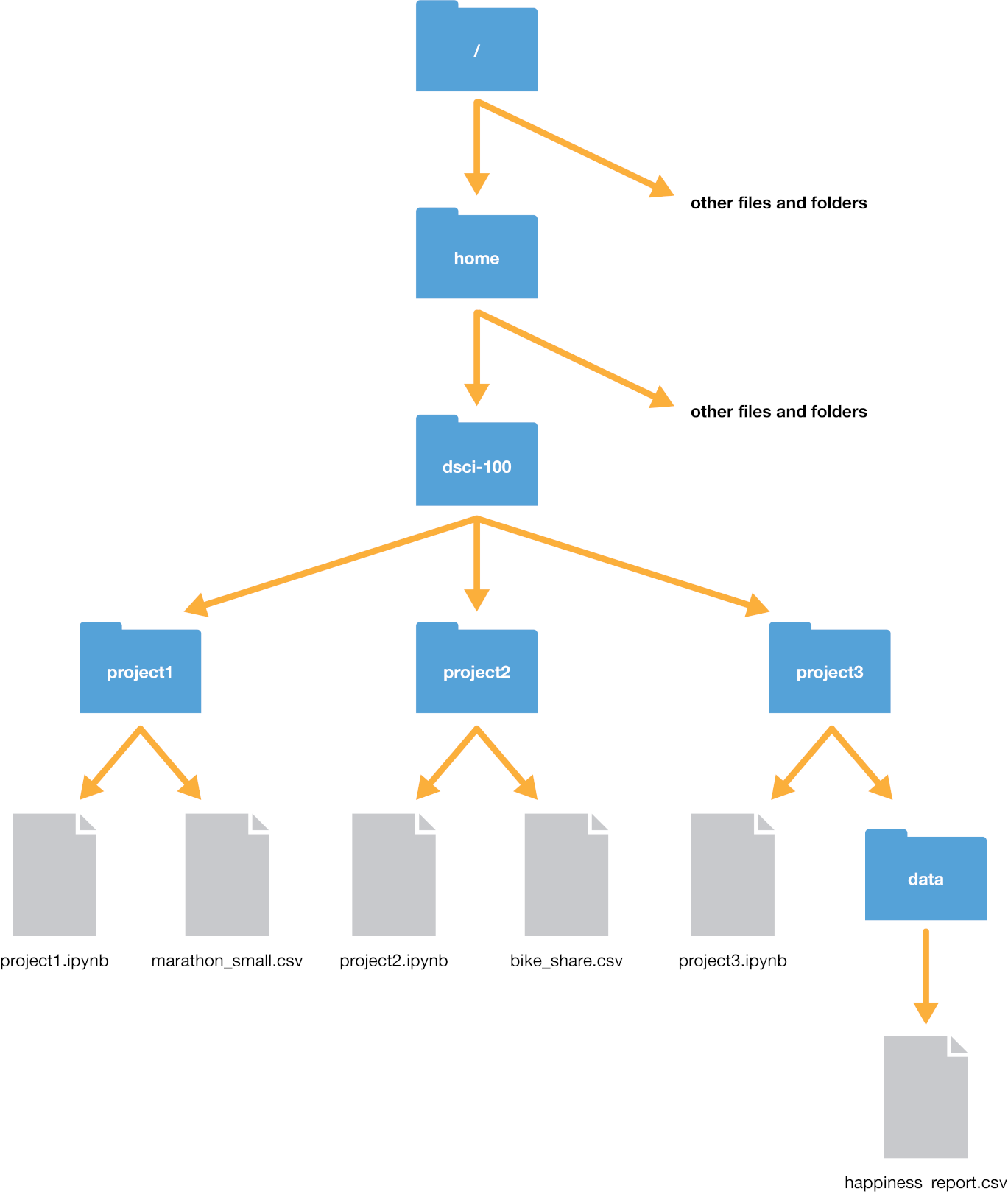
The place where your file lives is referred to as its ‘path’. You can think of the path as directions to the file. There are two kinds of paths: relative and absolute. A relative path indicates where a file is with respect to your working directory. An absolute path indicates where the file is with respect to the computers filesystem base (or root) folder, regardless of where you are working.

Example from Data Science: A first introduction with Python (link)

Here are some helpful shortcuts for file paths.

Symbol	Meaning
`~`	Home directory
`.`	Current working directory
`..`	One directory up from current working directory
`../..`	Two directories up from current working directory

Example: suppose we are in /home/dsci-100/project3. The location of happiness_report.csv relative to our current position is: - data/happiness_report.csv (you could also use ./data/happiness_report.csv with 1 dot, instead of 2!)

Best practices

In general, you should avoid using absolute file paths in your code, as these will never work on someone else’s computer.

A good workflow for a data analysis project is:

create a project directory (e.g. /Users/gm845/Library/2025/project1)
in project1, create a file structure - I like:
- src: this is where you put your code
- data: this is where you put your data
- doc: this is where you put your documents (e.g. Word or LaTex files)
- etc: miscellaneous files (e.g. pictures of whiteboards)

Within your project, you should use relative file paths. This makes your code portable if someone else copies your project1 folder.

In terms of naming your files, here are some good file naming practices from Jenny Bryan (link). Some key principles:

machine readable file names (easy to narrow file lists bases on names, or extract info from file names based on splitting, NO SPACES)
human readable file names (enough info to know what file is)
plays well with default ordering (e.g. zero pad files 01-exercise.py, 02-exercise.py, …, 11-exercise.py)

Loading data

In Lectures 2 and 3, we looked at the exchange rate data, which we read in as a .csv (comma separated value) file using pd.read_csv('../data/rates.csv').

Comma separated values files look like this:

a,b,c,d,message
1,2,3,4,hello
5,6,7,8,world
9,10,11,12,foo

import pandas as pd
import numpy as np
import seaborn as sns

ex1 = pd.read_csv('../data/example_01.csv')

ex1

	a	b	c	d	message
0	1	2	3	4	hello
1	5	6	7	8	world
2	9	10	11	12	foo

Suppose we do not have a header in the file - then, we can specify header=None:

ex2 = pd.read_csv('../data/example_02.csv', header=None)

Skipping rows

!cat ../data/example_03.csv

Here is a dataframe that we created:
(it is a simple example)
a,b,c,d,message
1,2,3,4,hello
5,6,7,8,world
9,10,11,12,foo

Note: Above, the ! allows shell commands to be run within cells. That is, in Terminal (or another shell), we can run cat ../data/example_03.csv to display the file.

Suppose we try to load example_03.csv:

# this gives an error 
# ex3 = pd.read_csv('../data/example_03.csv')

We don’t want the first 2 lines; we can use the argument skiprows to skip them when loading the data:

ex3 = pd.read_csv('../data/example_03.csv', skiprows=2)

ex3

	a	b	c	d	message
0	1	2	3	4	hello
1	5	6	7	8	world
2	9	10	11	12	foo

Using the `sep` argument for different separators

So far we have seen csv files. What about .txt files with tabs separating datapoints?

pd.read_csv('../data/example_04.txt', header=None)

	0
0	1\t2\t3\t4\thello
1	5\t6\t7\t8\tworld
2	9\t10\t11\t12\tfoo

ex4 = pd.read_csv('../data/example_04.txt', sep='\t', header=None)

ex4

	0	1	2	3	4
0	1	2	3	4	hello
1	5	6	7	8	world
2	9	10	11	12	foo

Note: \t is an example of an escaped character, which always starts with a backslash (\). Escaped characters are used to represent non-printing characters (like the tab or new line \n).

Note: there are lots of potential arguments for pd.read_csv. In Lecture 2, we saw the parse_dates argument as:

df = pd.read_csv('../data/rates.csv', parse_dates=['Time'])

The parse_dates argument takes a list of column names and tries to parse each of the columns as a date column.

The pd.read_csv arguments may fall into a few categories:

Indexing: Can treat one or more columns as the returned DataFrame, and whether to get column names from the file, arguments you provide, or not at all.
Type inference and data conversion: Includes the user-defined value conversions and custom list of missing value markers.
Date and time parsing: Includes a combining capability, including combining date and time information spread over multiple columns into a single column in the result.
Iterating: Support for iterating over chunks of very large files.
Unclean data issues: Includes skipping rows or a footer, comments, or other minor things like numeric data with thousands separated by commas.

For full information, you can see the documentation here.

Reading URLs

We can also read in data from a URL.

penguins = pd.read_csv("https://raw.githubusercontent.com/mwaskom/seaborn-data/master/penguins.csv")

penguins.head()

	species	island	bill_length_mm	bill_depth_mm	flipper_length_mm	body_mass_g	sex
0	Adelie	Torgersen	39.1	18.7	181.0	3750.0	MALE
1	Adelie	Torgersen	39.5	17.4	186.0	3800.0	FEMALE
2	Adelie	Torgersen	40.3	18.0	195.0	3250.0	FEMALE
3	Adelie	Torgersen	NaN	NaN	NaN	NaN	NaN
4	Adelie	Torgersen	36.7	19.3	193.0	3450.0	FEMALE

Reading Excel files

Gapminder is an independent education non-profit which releases public datasets (link).

We downloaded three datasets: - gdp_pcap.xlsx (Gross Domestic Product per capita) - lex.xlsx (Life expectancy) - pop.xlsx (Population)

Note: there are years past 2025 - these are projections, with details of projections in the documentation linked above.

The file name extension .xlsx refers to Microsoft Excel files, which store data very differently to csv or txt files:

PK?]Nd??xl/_rels/workbook.xml.rels<?xml version="1.0" encoding="UTF-8" standalone="yes"?>
(base) sas5ce91e6ae9a7:lec-4 gm845$ cat ../data/gdp_pcap.xlsx | head -n 2
PK?]Nd??xl/_rels/workbook.xml.rels<?xml version="1.0" encoding="UTF-8" standalone="yes"?>
<Relationships xmlns="http://schemas.openxmlformats.org/package/2006/relationships"><Relationship Id="rId1" Type="http://schemas.openxmlformats.org/officeDocument/2006/relationships/worksheet" Target="worksheets/sheet1.xml"/><Relationship Id="rId2" Type="http://schemas.openxmlformats.org/officeDocument/2006/relationships/sharedStrings" Target="sharedStrings.xml"/><Relationship Id="rId3"

To read this data, we use pd.read_excel. Note: you may need to install the openpyxl package in terminal (after activating your environment):

conda activate msds597
conda install openpyxl

and restart the VSCode python kernel.

gdp = pd.read_excel('../data/gdp_pcap.xlsx')
pop = pd.read_excel('../data/pop.xlsx')
lex = pd.read_excel('../data/lex.xlsx')

gdp.head()

	country	1800	1801	1802	1803	1804	1805	1806	1807	1808	...	2091	2092	2093	2094	2095	2096	2097	2098	2099	2100
0	Afghanistan	481	481	481	481	481	481	481	481	481	...	4680	4790	4910	5020	5140	5260	5380	5510	5640	5780
1	Angola	373	374	376	378	379	381	383	385	386	...	24.5k	25k	25.6k	26.1k	26.6k	27.1k	27.7k	28.2k	28.8k	29.3k
2	Albania	469	471	472	473	475	476	477	479	480	...	54.5k	55.1k	55.7k	56.3k	56.9k	57.4k	58k	58.6k	59.2k	59.8k
3	Andorra	1370	1370	1370	1380	1380	1380	1390	1390	1390	...	79.9k	80.2k	80.4k	80.7k	81k	81.3k	81.5k	81.8k	82k	82.3k
4	UAE	1140	1150	1150	1150	1160	1160	1170	1170	1180	...	92.6k	92.6k	92.6k	92.7k	92.7k	92.7k	92.8k	92.8k	92.8k	92.9k

5 rows × 302 columns

pop.head()

	country	1800	1801	1802	1803	1804	1805	1806	1807	1808	...	2091	2092	2093	2094	2095	2096	2097	2098	2099	2100
0	Afghanistan	3.28M	3.28M	3.28M	3.28M	3.28M	3.28M	3.28M	3.28M	3.28M	...	124M	125M	126M	126M	127M	128M	128M	129M	130M	130M
1	Angola	1.57M	1.57M	1.57M	1.57M	1.57M	1.57M	1.57M	1.57M	1.57M	...	139M	140M	142M	143M	144M	145M	147M	148M	149M	150M
2	Albania	400k	402k	404k	405k	407k	409k	411k	413k	414k	...	1.34M	1.32M	1.3M	1.29M	1.27M	1.25M	1.23M	1.22M	1.2M	1.18M
3	Andorra	2650	2650	2650	2650	2650	2650	2650	2650	2650	...	52.8k	52.1k	51.5k	50.8k	50.2k	49.6k	49k	48.4k	47.8k	47.2k
4	UAE	40.2k	40.2k	40.2k	40.2k	40.2k	40.2k	40.2k	40.2k	40.2k	...	24.1M	24.3M	24.5M	24.7M	25M	25.2M	25.4M	25.7M	25.9M	26.1M

5 rows × 302 columns

lex.head()

	country	1800	1801	1802	1803	1804	1805	1806	1807	1808	...	2091	2092	2093	2094	2095	2096	2097	2098	2099	2100
0	Afghanistan	28.2	28.2	28.2	28.2	28.2	28.2	28.1	28.1	28.1	...	75.9	76.1	76.2	76.4	76.5	76.7	76.8	77.0	77.1	77.3
1	Angola	27.0	27.0	27.0	27.0	27.0	27.0	27.0	27.0	27.0	...	75.8	75.9	76.0	76.1	76.3	76.4	76.5	76.7	76.8	76.9
2	Albania	35.4	35.4	35.4	35.4	35.4	35.4	35.4	35.4	35.4	...	88.9	89.0	89.2	89.3	89.4	89.5	89.6	89.7	89.8	90.0
3	Andorra	NaN	NaN	NaN	NaN	NaN	NaN	NaN	NaN	NaN	...	91.0	91.1	91.3	91.4	91.5	91.6	91.7	91.8	91.9	92.0
4	UAE	30.7	30.7	30.7	30.7	30.7	30.7	30.7	30.7	30.7	...	83.7	83.8	83.9	84.0	84.1	84.2	84.3	84.5	84.6	84.7

5 rows × 302 columns

Let’s practice some of our data skills from previous lectures.

Turn each dataset into tidy data

gdp = gdp.melt(id_vars='country',
         var_name='year',
         value_name='gdp')

gdp.head()

	country	year	gdp
0	Afghanistan	1800	481
1	Angola	1800	373
2	Albania	1800	469
3	Andorra	1800	1370
4	UAE	1800	1140

pop = pop.melt(id_vars = 'country',
               var_name = 'year',
               value_name = 'pop')

lex = lex.melt(id_vars = 'country',
               var_name = 'year',
               value_name = 'lex')

Merge the datasets together

gapminder = gdp.merge(pop, on=['country', 'year']).merge(lex, on=['country', 'year'])

gapminder.head()

	country	year	gdp	pop	lex
0	Afghanistan	1800	481	3.28M	28.2
1	Angola	1800	373	1.57M	27.0
2	Albania	1800	469	400k	35.4
3	Andorra	1800	1370	2650	NaN
4	UAE	1800	1140	40.2k	30.7

Keep only years 1950-2019

keep = (gapminder['year'] >= 1950) & (gapminder['year'] <= 2019)

# an alternative
keep = gapminder['year'].between(1950, 2019)

gapminder = gapminder[keep]

gapminder = gapminder.reset_index().drop(columns='index')

Are there any NaNs?

gapminder.isna().sum()

country    0
year       0
gdp        0
pop        0
lex        0
dtype: int64

String manipulation

Illustration: Gapminder data

We can still see some issues - numbers are in 14M and 14k formats and are read as strings, not integers or floats.

We can use Python string methods to clean this data.

First, let’s look at some of the data:

test = gapminder.loc[0, 'pop']

test

'7.78M'

isinstance(test, str)

True

Numbers in the millions are stored as strings.

test2 = gapminder.loc[3,'pop']

test2

type(test2)

int

We can iterate over strings:

for ch in test:
    print(ch)

7
.
7
8
M

For each string element, we can see if it’s a letter using .isalpha().

for ch in test:
    if ch.isalpha():
        print(ch)

Finally, let’s write our function that returns all the letters we may see in the pd.Series.

def get_number_formats(x):

    num_forms = []
    for val in x:
        if isinstance(val, str):
            for ch in val:
                if ch.isalpha():
                    num_forms.append(ch)

    return set(num_forms)

num_forms = get_number_formats(gapminder['pop'])

num_forms

{'B', 'M', 'k'}

Now, convert the strings to floats:

def convert_to_float(x):
    if isinstance(x, str):
        if 'k' in x:
            x_new = float(x.replace('k', '')) * 1000
        if 'M' in x:
            x_new = float(x.replace('M', '')) * 1000000
        if 'B' in x:
            x_new = float(x.replace('B', '')) * 1000000000

        return x_new
    
    else:
        return x

gapminder[['gdp', 'pop']] = gapminder[['gdp', 'pop']].map(convert_to_float)

gapminder['pop'] = gapminder['pop'].astype('int64')
gapminder['year'] = gapminder['year'].astype('int64')

year_plot = 2007
g = sns.relplot(gapminder[gapminder['year'] == year_plot],
            x='gdp',
            y='lex',
            size='pop',
            height = 4,
            aspect = 2)
g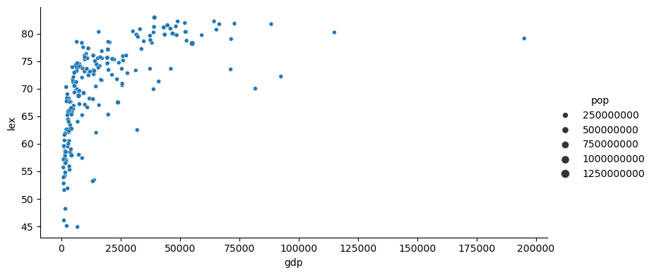

Let’s plot in log scale for the x-axis:

g = sns.relplot(gapminder[gapminder['year'] == year_plot],
            x='gdp',
            y='lex',
            size='pop',
            height = 4,
            aspect = 2)
g.set(xscale='log')
g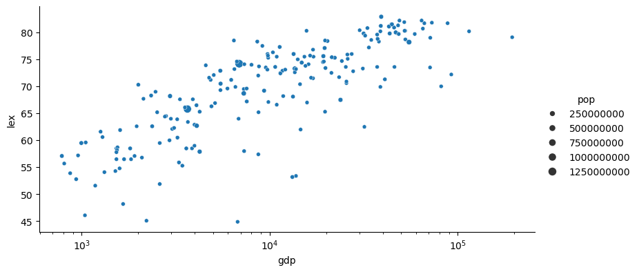

Above, we used the following Python built-in string methods:

.isalpha
.replace

Another helpful method is .split(), which breaks strings into a list of substrings using the passed delimiter:

my_string = '2,3,4,5'
my_string.split(',')

['2', '3', '4', '5']

String functions in pandas

We can apply string methods to pandas dataframes using pd.DataFrame.str.<method>.

Here is a list of some more helpful functions.

subset = gapminder['country'].str.contains('U')

gapminder['country'][subset].unique()

array(['UAE', 'UK', 'Uganda', 'Ukraine', 'Uruguay', 'USA', 'Uzbekistan'],
      dtype=object)

Standardizing Country Names

Let’s go back to our gapminder data! We are going to add continent data.

Install these packages in your msds597 environment:

Terminal

pip install pycountry
pip install pycountry_convert

import pycountry
import pycountry_convert as pc

df_country = gapminder[['country']].drop_duplicates()

df_country['country_code'] = pd.NA

df_country.dtypes

country         object
country_code    object
dtype: object

exceptions = []
for c in df_country['country']:
    try:
        df_country.loc[df_country['country']==c, 'country_code'] = pc.country_name_to_country_alpha2(c)
    except:
        exceptions.append(c)

exceptions

['UAE',
 "Cote d'Ivoire",
 'Congo, Dem. Rep.',
 'Congo, Rep.',
 'Micronesia, Fed. Sts.',
 'UK',
 'Hong Kong, China',
 'Lao',
 'St. Vincent and the Grenadines']

Let’s now do the painstaking work of finding exceptions:

uae = pycountry.countries.search_fuzzy('emirates')

uae

[Country(alpha_2='AE', alpha_3='ARE', flag='🇦🇪', name='United Arab Emirates', numeric='784')]

df_country['country'].str.contains('UAE')

0      False
1      False
2      False
3      False
4       True
       ...  
190    False
191    False
192    False
193    False
194    False
Name: country, Length: 195, dtype: bool

df_country.loc[df_country['country'].str.contains('UAE'), 'country_code'] = uae[0].alpha_2

ivoire = pycountry.countries.search_fuzzy('ivoire')

df_country.loc[df_country['country'].str.contains('Ivoire'), 'country_code'] = ivoire[0].alpha_2

congo = pycountry.countries.search_fuzzy('congo')

congo

[Country(alpha_2='CG', alpha_3='COG', flag='🇨🇬', name='Congo', numeric='178', official_name='Republic of the Congo'),
 Country(alpha_2='CD', alpha_3='COD', flag='🇨🇩', name='Congo, The Democratic Republic of the', numeric='180')]

df_country.loc[df_country['country'].str.contains('Congo, Dem.'), 'country_code'] = congo[1].alpha_2

df_country.loc[df_country['country'].str.contains('Congo, Rep.'), 'country_code'] = congo[0].alpha_2

mic = pycountry.countries.search_fuzzy('micronesia')

df_country.loc[df_country['country'].str.contains('Micronesia, Fed. Sts.'), 'country_code'] = mic[0].alpha_2

gb = pycountry.countries.search_fuzzy('great britain')

df_country.loc[df_country['country'].str.contains('UK'), 'country_code'] = gb[0].alpha_2

hk = pycountry.countries.search_fuzzy('hong kong')

df_country.loc[df_country['country'].str.contains('Hong Kong'), 'country_code'] = hk[0].alpha_2

laos = pycountry.countries.search_fuzzy('Laos')

df_country.loc[df_country['country'].str.contains('Lao'), 'country_code'] = laos[0].alpha_2

vin = pycountry.countries.search_fuzzy('Vincent')

df_country.loc[df_country['country'].str.contains('Vincent'), 'country_code'] = vin[0].alpha_2

Have we found them all?

any(df_country['country_code'].isna())

False

df_country['continent'] = pd.NA

exceptions = []
for c in df_country['country_code']:
    try:
        cc = pc.country_alpha2_to_continent_code(c)
        df_country.loc[df_country['country_code']==c, 'continent'] = pc.convert_continent_code_to_continent_name(cc)
    except:
        exceptions.append(c)

exceptions

['TL']

df_country.loc[df_country['country_code']=='TL', 'continent'] = 'Asia'

any(df_country['continent'].isna())

False

Merging continent data

gapminder = gapminder.merge(df_country, on='country')

gapminder.head()

	country	year	gdp	pop	lex	country_code	continent
0	Afghanistan	1950	1450.0	7780000	42.7	AF	Asia
1	Angola	1950	2230.0	4550000	45.6	AO	Africa
2	Albania	1950	1980.0	1250000	52.2	AL	Europe
3	Andorra	1950	8350.0	6000	74.6	AD	Europe
4	UAE	1950	1710.0	74500	58.4	AE	Asia

g = sns.relplot(gapminder[gapminder['year'] == year_plot],
            x='gdp',
            y='lex',
            size='pop',
            hue='continent',
            height = 4.5,
            aspect = 1.5)
g.set(xscale='log')
g.set_axis_labels("Gross Domestic Product per Capita", "Life Expectancy")
g.set(title=f'Gapminder Data (Year = {year_plot})')
g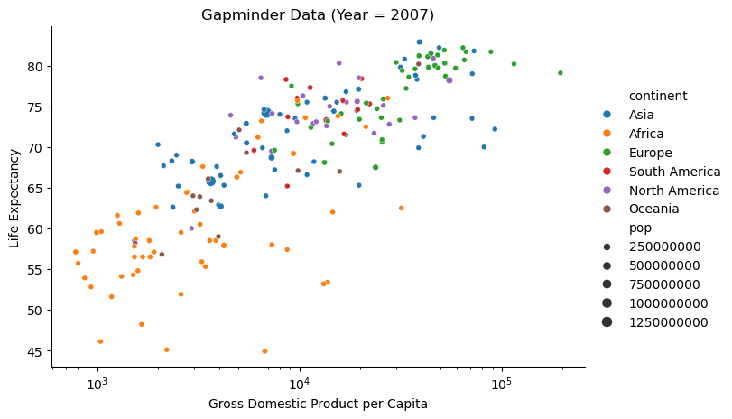

Illustration: World Health Organization Tuberculosis Data

We now consider another data cleaning exercise, adapted from R For Data Science (2e).

The data is who_data.csv, collected by the World Health Organisation (link). It contains information about tuberculosis diagnoses. The data contains:

country
year
56 columns like new_sp_m_014, new_ep_m_4554, and new_rel_m_3544.

Each of the 56 columns follow a pattern.

The first three letters of each column denote whether the column contains new or old cases of TB. In this dataset, each column contains new cases.
The next two letters describe the type of TB:

rel stands for cases of relapse
ep stands for cases of extrapulmonary TB
sn stands for cases of pulmonary TB that could not be diagnosed by a pulmonary smear (smear negative)
sp stands for cases of pulmonary TB that could be diagnosed by a pulmonary smear (smear positive)

The sixth letter gives the sex of TB patients. The dataset groups cases by males (m) and females (f).
The remaining numbers gives the age group. The dataset groups cases into seven age groups:

014 = 0 – 14 years old
1524 = 15 – 24 years old
2534 = 25 – 34 years old
3544 = 35 – 44 years old
4554 = 45 – 54 years old
5564 = 55 – 64 years old
65 = 65 or older

who = pd.read_csv('../data/who_data.csv')
who.head()

	country	iso2	iso3	year	new_sp_m014	new_sp_m1524	new_sp_m2534	new_sp_m3544	new_sp_m4554	new_sp_m5564	...	newrel_m4554	newrel_m5564	newrel_m65	newrel_f014	newrel_f1524	newrel_f2534	newrel_f3544	newrel_f4554	newrel_f5564	newrel_f65
0	Afghanistan	AF	AFG	1980	NaN	NaN	NaN	NaN	NaN	NaN	...	NaN	NaN	NaN	NaN	NaN	NaN	NaN	NaN	NaN	NaN
1	Afghanistan	AF	AFG	1981	NaN	NaN	NaN	NaN	NaN	NaN	...	NaN	NaN	NaN	NaN	NaN	NaN	NaN	NaN	NaN	NaN
2	Afghanistan	AF	AFG	1982	NaN	NaN	NaN	NaN	NaN	NaN	...	NaN	NaN	NaN	NaN	NaN	NaN	NaN	NaN	NaN	NaN
3	Afghanistan	AF	AFG	1983	NaN	NaN	NaN	NaN	NaN	NaN	...	NaN	NaN	NaN	NaN	NaN	NaN	NaN	NaN	NaN	NaN
4	Afghanistan	AF	AFG	1984	NaN	NaN	NaN	NaN	NaN	NaN	...	NaN	NaN	NaN	NaN	NaN	NaN	NaN	NaN	NaN	NaN

5 rows × 60 columns

Let’s first put the data in tidy form:

who_melt = who.melt(id_vars=['country', 'iso2', 'iso3', 'year'],
                    var_name='key',
                    value_name='cases')

who_melt.head()

	country	iso2	iso3	year	key	cases
0	Afghanistan	AF	AFG	1980	new_sp_m014	NaN
1	Afghanistan	AF	AFG	1981	new_sp_m014	NaN
2	Afghanistan	AF	AFG	1982	new_sp_m014	NaN
3	Afghanistan	AF	AFG	1983	new_sp_m014	NaN
4	Afghanistan	AF	AFG	1984	new_sp_m014	NaN

Let’s drop NaNs.

who_melt = who_melt.dropna()
who_melt.head()

	country	iso2	iso3	year	key	cases
17	Afghanistan	AF	AFG	1997	new_sp_m014	0.0
18	Afghanistan	AF	AFG	1998	new_sp_m014	30.0
19	Afghanistan	AF	AFG	1999	new_sp_m014	8.0
20	Afghanistan	AF	AFG	2000	new_sp_m014	52.0
21	Afghanistan	AF	AFG	2001	new_sp_m014	129.0

who_melt['key'].unique()

array(['new_sp_m014', 'new_sp_m1524', 'new_sp_m2534', 'new_sp_m3544',
       'new_sp_m4554', 'new_sp_m5564', 'new_sp_m65', 'new_sp_f014',
       'new_sp_f1524', 'new_sp_f2534', 'new_sp_f3544', 'new_sp_f4554',
       'new_sp_f5564', 'new_sp_f65', 'new_sn_m014', 'new_sn_m1524',
       'new_sn_m2534', 'new_sn_m3544', 'new_sn_m4554', 'new_sn_m5564',
       'new_sn_m65', 'new_sn_f014', 'new_sn_f1524', 'new_sn_f2534',
       'new_sn_f3544', 'new_sn_f4554', 'new_sn_f5564', 'new_sn_f65',
       'new_ep_m014', 'new_ep_m1524', 'new_ep_m2534', 'new_ep_m3544',
       'new_ep_m4554', 'new_ep_m5564', 'new_ep_m65', 'new_ep_f014',
       'new_ep_f1524', 'new_ep_f2534', 'new_ep_f3544', 'new_ep_f4554',
       'new_ep_f5564', 'new_ep_f65', 'newrel_m014', 'newrel_m1524',
       'newrel_m2534', 'newrel_m3544', 'newrel_m4554', 'newrel_m5564',
       'newrel_m65', 'newrel_f014', 'newrel_f1524', 'newrel_f2534',
       'newrel_f3544', 'newrel_f4554', 'newrel_f5564', 'newrel_f65'],
      dtype=object)

Looks like most keys have pattern new_type_sexage, except newrel. Let’s change that.

who_melt['key'] = who_melt['key'].str.replace('newrel', 'new_rel')

who_melt['key'].unique()

array(['new_sp_m014', 'new_sp_m1524', 'new_sp_m2534', 'new_sp_m3544',
       'new_sp_m4554', 'new_sp_m5564', 'new_sp_m65', 'new_sp_f014',
       'new_sp_f1524', 'new_sp_f2534', 'new_sp_f3544', 'new_sp_f4554',
       'new_sp_f5564', 'new_sp_f65', 'new_sn_m014', 'new_sn_m1524',
       'new_sn_m2534', 'new_sn_m3544', 'new_sn_m4554', 'new_sn_m5564',
       'new_sn_m65', 'new_sn_f014', 'new_sn_f1524', 'new_sn_f2534',
       'new_sn_f3544', 'new_sn_f4554', 'new_sn_f5564', 'new_sn_f65',
       'new_ep_m014', 'new_ep_m1524', 'new_ep_m2534', 'new_ep_m3544',
       'new_ep_m4554', 'new_ep_m5564', 'new_ep_m65', 'new_ep_f014',
       'new_ep_f1524', 'new_ep_f2534', 'new_ep_f3544', 'new_ep_f4554',
       'new_ep_f5564', 'new_ep_f65', 'new_rel_m014', 'new_rel_m1524',
       'new_rel_m2534', 'new_rel_m3544', 'new_rel_m4554', 'new_rel_m5564',
       'new_rel_m65', 'new_rel_f014', 'new_rel_f1524', 'new_rel_f2534',
       'new_rel_f3544', 'new_rel_f4554', 'new_rel_f5564', 'new_rel_f65'],
      dtype=object)

How to split up these keys?

who_melt['key'].str.split('_')

17        [new, sp, m014]
18        [new, sp, m014]
19        [new, sp, m014]
20        [new, sp, m014]
21        [new, sp, m014]
               ...       
405269    [new, rel, f65]
405303    [new, rel, f65]
405371    [new, rel, f65]
405405    [new, rel, f65]
405439    [new, rel, f65]
Name: key, Length: 75752, dtype: object

who_split = who_melt['key'].str.split('_', expand=True)
who_split

	0	1	2
17	new	sp	m014
18	new	sp	m014
19	new	sp	m014
20	new	sp	m014
21	new	sp	m014
...	...	...	...
405269	new	rel	f65
405303	new	rel	f65
405371	new	rel	f65
405405	new	rel	f65
405439	new	rel	f65

75752 rows × 3 columns

Change column names:

who_split.columns = ['new', 'type', 'sexage']

Split sexage into sex and age columns:

who_split['sexage'].str.slice(start=0, stop=1)

17        m
18        m
19        m
20        m
21        m
         ..
405269    f
405303    f
405371    f
405405    f
405439    f
Name: sexage, Length: 75752, dtype: object

who_split['sex'] = who_split['sexage'].str.slice(start=0, stop=1)

who_split['age'] = who_split['sexage'].str.slice(start=1)

who_split.head()

	new	type	sexage	sex	age
17	new	sp	m014	m	014
18	new	sp	m014	m	014
19	new	sp	m014	m	014
20	new	sp	m014	m	014
21	new	sp	m014	m	014
...	...	...	...	...	...
405269	new	rel	f65	f	65
405303	new	rel	f65	f	65
405371	new	rel	f65	f	65
405405	new	rel	f65	f	65
405439	new	rel	f65	f	65

75752 rows × 5 columns

In this dataset, all cases are new:

who_split['new'].unique()

array(['new'], dtype=object)

who_split = who_split.drop(columns=['new', 'sexage'])

who_split['age'] = who_split['age'].astype('category')

who_split['age'] = who_split['age'].cat.as_ordered()

who_split['age']

17        014
18        014
19        014
20        014
21        014
         ... 
405269     65
405303     65
405371     65
405405     65
405439     65
Name: age, Length: 75752, dtype: category
Categories (7, object): ['014' < '1524' < '2534' < '3544' < '4554' < '5564' < '65']

who_split.head()

	type	sex	age
17	sp	m	014
18	sp	m	014
19	sp	m	014
20	sp	m	014
21	sp	m	014

who_tidy = who_melt.merge(who_split, left_index=True, right_index=True)
who_tidy.head()

	country	iso2	iso3	year	key	cases	type	sex	age
17	Afghanistan	AF	AFG	1997	new_sp_m014	0.0	sp	m	014
18	Afghanistan	AF	AFG	1998	new_sp_m014	30.0	sp	m	014
19	Afghanistan	AF	AFG	1999	new_sp_m014	8.0	sp	m	014
20	Afghanistan	AF	AFG	2000	new_sp_m014	52.0	sp	m	014
21	Afghanistan	AF	AFG	2001	new_sp_m014	129.0	sp	m	014

who_tidy = who_tidy.drop(columns=['key'])

who_tidy.head()

	country	iso2	iso3	year	cases	type	sex	age
17	Afghanistan	AF	AFG	1997	0.0	sp	m	014
18	Afghanistan	AF	AFG	1998	30.0	sp	m	014
19	Afghanistan	AF	AFG	1999	8.0	sp	m	014
20	Afghanistan	AF	AFG	2000	52.0	sp	m	014
21	Afghanistan	AF	AFG	2001	129.0	sp	m	014

sns.relplot(who_tidy[who_tidy.iso2 == 'AF'],
            x='year',
            y='cases',
            hue='type',
            style='sex',
            col='age',
            col_wrap=3)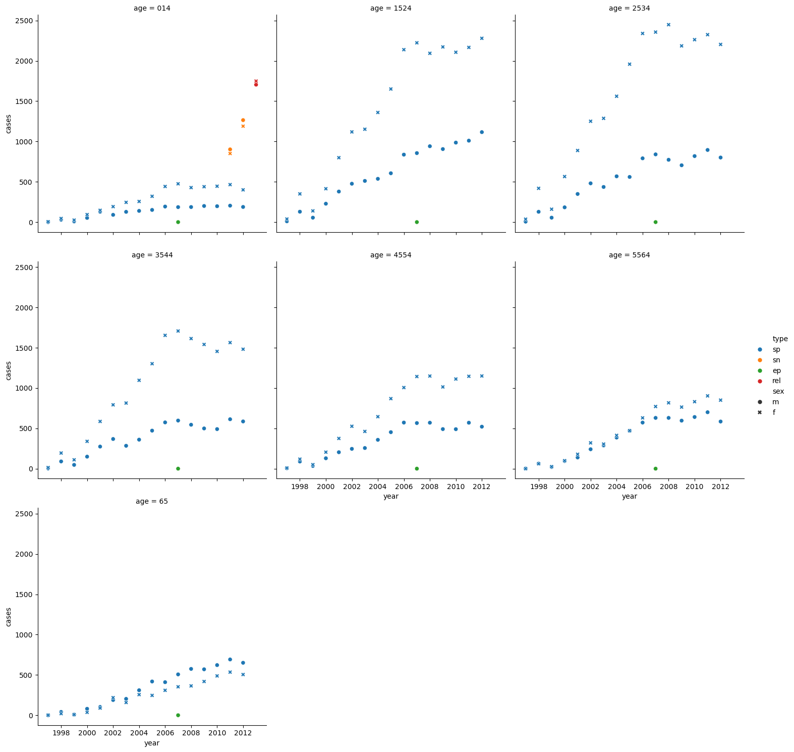

Internet data types

JSON data

JSON (short for JavaScript Object Notation) is a standard format for sending data by HTTP request between web browsers and other applications.

Here is an example from NYC Open Data

The data is on Citi-Bike Stations in NYC, and the start of it looks like:

{"data": {"stations": [{"is_installed": 0, "is_returning": 0, "num_bikes_disabled": 0, "is_renting": 0, "station_id": "1817822909864556798", "num_docks_disabled": 0, "legacy_id": "1817822909864556798", "last_reported": 1739366429, "num_ebikes_available": 0, "num_bikes_available": 0, "num_docks_available": 0, "eightd_has_available_keys": false}, {"is_installed": 1, "is_returning": 1, "num_bikes_disabled": 4, "is_renting": 1, "station_id": "5a24acbb-94ef-4cb5-9db8-f6073ac26a2b", "num_docks_disabled": 0, "legacy_id": "4302", "num_scooters_available": 0, "last_reported": 1739394755, "num_ebikes_available": 0,

We can see it looks nearly like valid Python code (e.g. a dictionary).

A helpful package for reading JSON data is json:

import json

bike_data = json.load(open('../data/citibike.json'))

bike_data.keys()

dict_keys(['data', 'last_updated', 'ttl', 'version'])

bike_data['data'].keys()

dict_keys(['stations'])

stations = pd.DataFrame(bike_data['data']['stations'])

stations.head()

	is_installed	is_returning	num_bikes_disabled	is_renting	station_id	legacy_id	last_reported	num_ebikes_available	num_bikes_available	num_docks_available	eightd_has_available_keys	num_scooters_available	num_scooters_unavailable
0	0	0	0	0	1817822909864556798	1817822909864556798	1739366429	0	0	0	False	NaN	NaN
1	1	1	1	1	bacfe3c2-7946-45ed-91f9-f5b91791de75	3503	1739395003	1	2	27	False	0.0	0.0
2	1	1	5	1	9394fb49-583f-4426-8d2f-a2b0ffb584d2	3737	1739395004	4	34	10	False	0.0	0.0
3	1	1	9	1	1869753654337059182	1869753654337059182	1739394999	1	10	2	False	0.0	0.0
4	1	1	6	1	1f8f6714-42a7-45d5-86cd-a093c940b2c9	4635	1739395000	1	2	19	False	0.0	0.0

HTML data

To read in HTML tables, for example, we can use the pd.read_html command.

Note: we need the following packages:

conda install lxml beautifulsoup4 html5lib

This is because pd.read_html uses lxml or Beautiful Soup under the hood to parse data from HTML.

The following is from the pandas documenation, and gets a table of failed banks from the FDIC website.

url = "https://www.fdic.gov/resources/resolutions/bank-failures/failed-bank-list"
banks = pd.read_html(url)

type(banks)

list

Note: pd.read_html reads HTML tables into a list of DataFrame objects. This is helpful if there is more than one table on the website.

banks[0]

	Bank Name	City	State	Cert	Aquiring Institution	Closing Date	Fund Sort ascending
0	Pulaski Savings Bank	Chicago	Illinois	28611	Millennium Bank	January 17, 2025	10548
1	The First National Bank of Lindsay	Lindsay	Oklahoma	4134	First Bank & Trust Co., Duncan, OK	October 18, 2024	10547
2	Republic First Bank dba Republic Bank	Philadelphia	Pennsylvania	27332	Fulton Bank, National Association	April 26, 2024	10546
3	Citizens Bank	Sac City	Iowa	8758	Iowa Trust & Savings Bank	November 3, 2023	10545
4	Heartland Tri-State Bank	Elkhart	Kansas	25851	Dream First Bank, N.A.	July 28, 2023	10544
5	First Republic Bank	San Francisco	California	59017	JPMorgan Chase Bank, N.A.	May 1, 2023	10543
6	Signature Bank	New York	New York	57053	Flagstar Bank, N.A.	March 12, 2023	10540
7	Silicon Valley Bank	Santa Clara	California	24735	First Citizens Bank & Trust Company	March 10, 2023	10539
8	Almena State Bank	Almena	Kansas	15426	Equity Bank	October 23, 2020	10538
9	First City Bank of Florida	Fort Walton Beach	Florida	16748	United Fidelity Bank, fsb	October 16, 2020	10537

XML data

XML is another common structured data format supporting hierarchical, nested data with metadata. XML and HTML are similar, but XML is more general.

The following is an example from the xml.etree.ElementTree documentation.

!cat ../data/country_data.xml

<?xml version="1.0"?>
<data>
    <country name="Liechtenstein">
        <rank>1</rank>
        <year>2008</year>
        <gdppc>141100</gdppc>
        <neighbor name="Austria" direction="E"/>
        <neighbor name="Switzerland" direction="W"/>
    </country>
    <country name="Singapore">
        <rank>4</rank>
        <year>2011</year>
        <gdppc>59900</gdppc>
        <neighbor name="Malaysia" direction="N"/>
    </country>
    <country name="Panama">
        <rank>68</rank>
        <year>2011</year>
        <gdppc>13600</gdppc>
        <neighbor name="Costa Rica" direction="W"/>
        <neighbor name="Colombia" direction="E"/>
    </country>
</data>

import xml.etree.ElementTree as ET

tree = ET.parse('../data/country_data.xml')
root = tree.getroot()

XML documents are represented as a tree of elements

Each element has:

a tag (name)
attributes (optional)
text content (optional)

root.tag

'data'

root.attrib

{}

for child in root:
    print(child.tag, child.attrib, child.text)
    for child2 in child:
        print('--', child2.tag, child2.attrib, child2.text)
    print('\n')

country {'name': 'Liechtenstein'} 
        
-- rank {} 1
-- year {} 2008
-- gdppc {} 141100
-- neighbor {'name': 'Austria', 'direction': 'E'} None
-- neighbor {'name': 'Switzerland', 'direction': 'W'} None


country {'name': 'Singapore'} 
        
-- rank {} 4
-- year {} 2011
-- gdppc {} 59900
-- neighbor {'name': 'Malaysia', 'direction': 'N'} None


country {'name': 'Panama'} 
        
-- rank {} 68
-- year {} 2011
-- gdppc {} 13600
-- neighbor {'name': 'Costa Rica', 'direction': 'W'} None
-- neighbor {'name': 'Colombia', 'direction': 'E'} None

We can access elements using indexing:

root[0]

<Element 'country' at 0x3064bb830>

root[0].attrib

{'name': 'Liechtenstein'}

root[0].attrib['name']

'Liechtenstein'

# We can also use .get to extract a specific attribute value
root[0].get('name')

'Liechtenstein'

# We can use .find to get the first matching subelement
root[0].find('rank')

<Element 'rank' at 0x3064b9990>

# .find only works one subelement down - use the path for deeper elements
root.find('country/rank')

<Element 'rank' at 0x3064b9990>

# if you don't know the path, use './/tag_name'
root.find('.//rank')

<Element 'rank' at 0x3064b9990>

# We can use .find to get a list of all matching subelements
root.findall('.//rank')

[<Element 'rank' at 0x3064b9990>,
 <Element 'rank' at 0x3064b84f0>,
 <Element 'rank' at 0x306499cb0>]

You can also use pd.read_xml, however, this method is best designed to import shallow XML documents.

This function will always return a single DataFrame or raise exceptions due to issues with XML document, xpath, or other parameters.

xml_df = pd.read_xml('../data/country_data.xml')

xml_df

	name	rank	year	gdppc	neighbor
0	Liechtenstein	1	2008	141100	NaN
1	Singapore	4	2011	59900	NaN
2	Panama	68	2011	13600	NaN

Note that we lose the neighbor information.

More specifically, these are the kinds of formats easiest to read with pd.read_xml

<root>
    <row>
      <column1>data</column1>
      <column2>data</column2>
      <column3>data</column3>
      ...
   </row>
   <row>
      ...
   </row>
   ...
</root>

Illustration: Exchange Rate Data

Let’s look again at the exchange rate data from Lectures 2 and 3, but this time in XML form.

df = pd.read_xml('../data/eurofxref-hist-90d.xml')

df

	subject	name	Cube
0	Reference rates	None	None
1	None	European Central Bank	None
2	None	None	\n

The structure is too complicated to be directly read with pd.read_xml.

tree = ET.parse('../data/eurofxref-hist-90d.xml')
root = tree.getroot()
root.tag

'{http://www.gesmes.org/xml/2002-08-01}Envelope'

for child in root:
    print(child.tag, child.attrib, child.text)

{http://www.gesmes.org/xml/2002-08-01}subject {} Reference rates
{http://www.gesmes.org/xml/2002-08-01}Sender {} 
    
{http://www.ecb.int/vocabulary/2002-08-01/eurofxref}Cube {}

for child in root:
    print(child.tag, child.attrib, child.text)
    for i, child2 in enumerate(child):
        if i < 5:
            print('---', child2.tag, child2.attrib, child2.text)

{http://www.gesmes.org/xml/2002-08-01}subject {} Reference rates
{http://www.gesmes.org/xml/2002-08-01}Sender {} 
    
--- {http://www.gesmes.org/xml/2002-08-01}name {} European Central Bank
{http://www.ecb.int/vocabulary/2002-08-01/eurofxref}Cube {} 
    
--- {http://www.ecb.int/vocabulary/2002-08-01/eurofxref}Cube {'time': '2024-04-16'} 
      
--- {http://www.ecb.int/vocabulary/2002-08-01/eurofxref}Cube {'time': '2024-04-15'} 
      
--- {http://www.ecb.int/vocabulary/2002-08-01/eurofxref}Cube {'time': '2024-04-12'} 
      
--- {http://www.ecb.int/vocabulary/2002-08-01/eurofxref}Cube {'time': '2024-04-11'} 
      
--- {http://www.ecb.int/vocabulary/2002-08-01/eurofxref}Cube {'time': '2024-04-10'}

root[2].tag

'{http://www.ecb.int/vocabulary/2002-08-01/eurofxref}Cube'

cube = root[2]

for i, child in enumerate(cube):
    if i < 5:
        print(child.attrib)
        for j, child2 in enumerate(child):
            if j < 5:
                print('----', child2.attrib)

{'time': '2024-04-16'}
---- {'currency': 'USD', 'rate': '1.0637'}
---- {'currency': 'JPY', 'rate': '164.54'}
---- {'currency': 'BGN', 'rate': '1.9558'}
---- {'currency': 'CZK', 'rate': '25.21'}
---- {'currency': 'DKK', 'rate': '7.4609'}
{'time': '2024-04-15'}
---- {'currency': 'USD', 'rate': '1.0656'}
---- {'currency': 'JPY', 'rate': '164.05'}
---- {'currency': 'BGN', 'rate': '1.9558'}
---- {'currency': 'CZK', 'rate': '25.324'}
---- {'currency': 'DKK', 'rate': '7.4606'}
{'time': '2024-04-12'}
---- {'currency': 'USD', 'rate': '1.0652'}
---- {'currency': 'JPY', 'rate': '163.16'}
---- {'currency': 'BGN', 'rate': '1.9558'}
---- {'currency': 'CZK', 'rate': '25.337'}
---- {'currency': 'DKK', 'rate': '7.4603'}
{'time': '2024-04-11'}
---- {'currency': 'USD', 'rate': '1.0729'}
---- {'currency': 'JPY', 'rate': '164.18'}
---- {'currency': 'BGN', 'rate': '1.9558'}
---- {'currency': 'CZK', 'rate': '25.392'}
---- {'currency': 'DKK', 'rate': '7.4604'}
{'time': '2024-04-10'}
---- {'currency': 'USD', 'rate': '1.086'}
---- {'currency': 'JPY', 'rate': '164.89'}
---- {'currency': 'BGN', 'rate': '1.9558'}
---- {'currency': 'CZK', 'rate': '25.368'}
---- {'currency': 'DKK', 'rate': '7.4594'}

cube[0][0].attrib['currency']

'USD'

cube[0][0].attrib['rate']

'1.0637'

xml_dict = {}

for i, child in enumerate(cube):
    temp_dict = {}
    for j, child2 in enumerate(child):
        temp_dict[child2.attrib['currency']] = child2.attrib['rate']
    xml_dict[child.attrib['time']] = temp_dict

df_xml = pd.DataFrame(xml_dict)

df_xml.head()

	2024-04-16	2024-04-15	2024-04-12	2024-04-11	2024-04-10	2024-04-09	2024-04-08	2024-04-05	2024-04-04	2024-04-03	...	2024-01-31	2024-01-30	2024-01-29	2024-01-26	2024-01-25	2024-01-24	2024-01-23	2024-01-22	2024-01-19	2024-01-18
USD	1.0637	1.0656	1.0652	1.0729	1.086	1.0867	1.0823	1.0841	1.0852	1.0783	...	1.0837	1.0846	1.0823	1.0871	1.0893	1.0905	1.0872	1.089	1.0887	1.0875
JPY	164.54	164.05	163.16	164.18	164.89	164.97	164.43	164.1	164.69	163.66	...	160.19	159.97	160.13	160.62	160.81	160.46	160.88	160.95	161.17	160.89
BGN	1.9558	1.9558	1.9558	1.9558	1.9558	1.9558	1.9558	1.9558	1.9558	1.9558	...	1.9558	1.9558	1.9558	1.9558	1.9558	1.9558	1.9558	1.9558	1.9558	1.9558
CZK	25.21	25.324	25.337	25.392	25.368	25.38	25.354	25.286	25.322	25.352	...	24.891	24.831	24.806	24.748	24.756	24.786	24.824	24.758	24.813	24.734
DKK	7.4609	7.4606	7.4603	7.4604	7.4594	7.459	7.4588	7.459	7.4589	7.4589	...	7.455	7.4543	7.4538	7.4549	7.456	7.4568	7.4574	7.4585	7.4575	7.4571

5 rows × 62 columns

df_xml = df_xml.T

df_xml.head()

	USD	JPY	BGN	CZK	DKK	GBP	HUF	PLN	RON	SEK	...	ILS	INR	KRW	MXN	MYR	NZD	PHP	SGD	THB	ZAR
2024-04-16	1.0637	164.54	1.9558	25.21	7.4609	0.8544	394.63	4.3435	4.9764	11.635	...	4.0001	88.8975	1481.62	17.9141	5.0973	1.8072	60.561	1.4509	38.958	20.2104
2024-04-15	1.0656	164.05	1.9558	25.324	7.4606	0.85405	394.25	4.2938	4.9742	11.5583	...	3.9578	88.895	1473.79	17.6561	5.0925	1.7943	60.558	1.4498	39.124	20.2067
2024-04-12	1.0652	163.16	1.9558	25.337	7.4603	0.85424	391.63	4.2603	4.9717	11.5699	...	4.0175	88.914	1469.79	17.5982	5.081	1.7872	60.256	1.4478	38.853	19.9907
2024-04-11	1.0729	164.18	1.9558	25.392	7.4604	0.85525	389.8	4.257	4.9713	11.531	...	4.03	89.4385	1469.32	17.6448	5.0936	1.792	60.577	1.4518	39.22	20.1614
2024-04-10	1.086	164.89	1.9558	25.368	7.4594	0.85515	389.18	4.2563	4.969	11.4345	...	4.0324	90.3585	1467.33	17.7305	5.1558	1.7856	61.408	1.4605	39.536	20.0851

5 rows × 30 columns

df_xml.index.name = 'Time'

df_xml = df_xml.reset_index()

df_xml.head()

	Time	USD	JPY	BGN	CZK	DKK	GBP	HUF	PLN	RON	...	ILS	INR	KRW	MXN	MYR	NZD	PHP	SGD	THB	ZAR
0	2024-04-16	1.0637	164.54	1.9558	25.21	7.4609	0.8544	394.63	4.3435	4.9764	...	4.0001	88.8975	1481.62	17.9141	5.0973	1.8072	60.561	1.4509	38.958	20.2104
1	2024-04-15	1.0656	164.05	1.9558	25.324	7.4606	0.85405	394.25	4.2938	4.9742	...	3.9578	88.895	1473.79	17.6561	5.0925	1.7943	60.558	1.4498	39.124	20.2067
2	2024-04-12	1.0652	163.16	1.9558	25.337	7.4603	0.85424	391.63	4.2603	4.9717	...	4.0175	88.914	1469.79	17.5982	5.081	1.7872	60.256	1.4478	38.853	19.9907
3	2024-04-11	1.0729	164.18	1.9558	25.392	7.4604	0.85525	389.8	4.257	4.9713	...	4.03	89.4385	1469.32	17.6448	5.0936	1.792	60.577	1.4518	39.22	20.1614
4	2024-04-10	1.086	164.89	1.9558	25.368	7.4594	0.85515	389.18	4.2563	4.969	...	4.0324	90.3585	1467.33	17.7305	5.1558	1.7856	61.408	1.4605	39.536	20.0851

5 rows × 31 columns

df_xml['Time'] = pd.to_datetime(df_xml['Time'])

df_xml = df_xml.melt(id_vars=['Time'],
                     var_name = 'currency',
                     value_name='rate')

df_xml

	Time	currency	rate
0	2024-04-16	USD	1.0637
1	2024-04-15	USD	1.0656
2	2024-04-12	USD	1.0652
3	2024-04-11	USD	1.0729
4	2024-04-10	USD	1.086
...	...	...	...
1855	2024-01-24	ZAR	20.5366
1856	2024-01-23	ZAR	20.7022
1857	2024-01-22	ZAR	20.8846
1858	2024-01-19	ZAR	20.6892
1859	2024-01-18	ZAR	20.597

1860 rows × 3 columns

Overview

References

Directories

Best practices

Loading data

Skipping rows

Using the sep argument for different separators

Reading URLs

Reading Excel files

String manipulation

Illustration: Gapminder data

String functions in pandas

Standardizing Country Names

Merging continent data

Illustration: World Health Organization Tuberculosis Data

Internet data types

JSON data

HTML data

XML data

Illustration: Exchange Rate Data

Using the `sep` argument for different separators