# Import packages
import numpy as np
import pandas as pd
import seaborn as snsLecture 2 - Introduction to Pandas
Overview
This lecture provides an introduction to Pandas, a Python package with structures and data manipulation tools designed to make data cleaning and analysis fast and convenient. Topics include:
- Pandas objects (
pd.Series,pd.DataFrame) - Essential pandas functionality (indexing, selection, filtering, operations on dataframes)
- The concept of tidy data (Wickham, 2014)
References
This lecture contains material from:
- Chapter 5, Python for Data Analysis, 3E (Wes McKinney, 2022)
- Pierre Bellec’s notes
About Pandas
Pandas is the Python module that provides functionality similar to R’s built-in data.frame object. Pandas is designed for working with tabular or heterogeneous data.
Pandas Series
A Series is a one-dimensional array-like object containing a sequence of values (of similar types to NumPy types) of the same type and an associated array of data labels, called its index.
s = pd.Series([2, 4, -1, 5])
s
0 2
1 4
2 -1
3 5
dtype: int64s.array<NumpyExtensionArray>
[np.int64(2), np.int64(4), np.int64(-1), np.int64(5)]
Length: 4, dtype: int64s.indexRangeIndex(start=0, stop=4, step=1)s = pd.Series([2, 4, -1, 5], index=['a', 'b', 'c', 'd'])s.indexIndex(['a', 'b', 'c', 'd'], dtype='object')s['a']np.int64(2)s[['a', 'd']]a 2
d 5
dtype: int64s * 2a 4
b 8
c -2
d 10
dtype: int64s[s>2]b 4
d 5
dtype: int64We can create a series from a numpy array:
# Creating a numpy array
a = np.arange(6, 15, 1) + 0.2
print(a.shape)
a(9,)array([ 6.2, 7.2, 8.2, 9.2, 10.2, 11.2, 12.2, 13.2, 14.2])s_from_np = pd.Series(a)
s_from_np0 6.2
1 7.2
2 8.2
3 9.2
4 10.2
5 11.2
6 12.2
7 13.2
8 14.2
dtype: float64s_from_np.array<NumpyExtensionArray>
[ np.float64(6.2), np.float64(7.2), np.float64(8.2), np.float64(9.2),
np.float64(10.2), np.float64(11.2), np.float64(12.2), np.float64(13.2),
np.float64(14.2)]
Length: 9, dtype: float64s_from_np.indexRangeIndex(start=0, stop=9, step=1)We can adjust the index in place:
s_from_np.index = [2 * i for i in range(len(s_from_np))]s_from_np0 6.2
2 7.2
4 8.2
6 9.2
8 10.2
10 11.2
12 12.2
14 13.2
16 14.2
dtype: float64Finally, we can turn the Series object back to an ndarray as:
s_from_np.to_numpy()array([ 6.2, 7.2, 8.2, 9.2, 10.2, 11.2, 12.2, 13.2, 14.2])We can also create a series from a dictionary:
dat = {"Ohio": 35000, "Texas": 71000, "Oregon": 16000, "Utah": 5000}
s_from_dict = pd.Series(dat)
s_from_dict
Ohio 35000
Texas 71000
Oregon 16000
Utah 5000
dtype: int64s_from_dict.to_dict(){'Ohio': 35000, 'Texas': 71000, 'Oregon': 16000, 'Utah': 5000}states = ["California", "Ohio", "Oregon", "Texas"]s_new = pd.Series(dat, index=states)s_newCalifornia NaN
Ohio 35000.0
Oregon 16000.0
Texas 71000.0
dtype: float64pd.isna(s_new)California True
Ohio False
Oregon False
Texas False
dtype: boolpd.notna(s_new)California False
Ohio True
Oregon True
Texas True
dtype: bools_new.isna()California True
Ohio False
Oregon False
Texas False
dtype: boolPandas DataFrame
A DataFrame represents a rectangular table of data and contains an ordered, named collection of columns, each of which can be a different value type (numeric, string, Boolean, etc.). The DataFrame has both a row and column index; it can be thought of as a dictionary of Series all sharing the same index.
data = {"state": ["Ohio", "Ohio", "Ohio", "Nevada", "Nevada", "Nevada"],
"year": [2000, 2001, 2002, 2001, 2002, 2003],
"pop": [1.5, 1.7, 3.6, 2.4, 2.9, 3.2]}
frame = pd.DataFrame(data)frame| state | year | pop | |
|---|---|---|---|
| 0 | Ohio | 2000 | 1.5 |
| 1 | Ohio | 2001 | 1.7 |
| 2 | Ohio | 2002 | 3.6 |
| 3 | Nevada | 2001 | 2.4 |
| 4 | Nevada | 2002 | 2.9 |
| 5 | Nevada | 2003 | 3.2 |
# adding a column (similar to dictionaries)
frame['debt'] = 16frame| state | year | pop | debt | |
|---|---|---|---|---|
| 0 | Ohio | 2000 | 1.5 | 16 |
| 1 | Ohio | 2001 | 1.7 | 16 |
| 2 | Ohio | 2002 | 3.6 | 16 |
| 3 | Nevada | 2001 | 2.4 | 16 |
| 4 | Nevada | 2002 | 2.9 | 16 |
| 5 | Nevada | 2003 | 3.2 | 16 |
len(frame)6frame['debt'] = np.linspace(16,20,num=len(frame))
frame| state | year | pop | debt | |
|---|---|---|---|---|
| 0 | Ohio | 2000 | 1.5 | 16.0 |
| 1 | Ohio | 2001 | 1.7 | 16.8 |
| 2 | Ohio | 2002 | 3.6 | 17.6 |
| 3 | Nevada | 2001 | 2.4 | 18.4 |
| 4 | Nevada | 2002 | 2.9 | 19.2 |
| 5 | Nevada | 2003 | 3.2 | 20.0 |
# another example
A2d = np.random.normal(size=(8, 2))
A2d.shape
(8, 2)df_from_np = pd.DataFrame(A2d)
df_from_np| 0 | 1 | |
|---|---|---|
| 0 | -2.372890 | 0.461543 |
| 1 | -0.280463 | 1.104957 |
| 2 | -0.078033 | -0.759848 |
| 3 | 1.013987 | 0.562257 |
| 4 | 0.168685 | 0.785529 |
| 5 | -0.862294 | -0.784686 |
| 6 | -1.642501 | -0.204560 |
| 7 | 0.056823 | 0.733871 |
df_from_np.head()| 0 | 1 | |
|---|---|---|
| 0 | -2.372890 | 0.461543 |
| 1 | -0.280463 | 1.104957 |
| 2 | -0.078033 | -0.759848 |
| 3 | 1.013987 | 0.562257 |
| 4 | 0.168685 | 0.785529 |
df_from_np.tail()| 0 | 1 | |
|---|---|---|
| 3 | 1.013987 | 0.562257 |
| 4 | 0.168685 | 0.785529 |
| 5 | -0.862294 | -0.784686 |
| 6 | -1.642501 | -0.204560 |
| 7 | 0.056823 | 0.733871 |
df_from_np.to_numpy()array([[-2.37288997, 0.4615429 ],
[-0.28046288, 1.10495676],
[-0.07803338, -0.75984847],
[ 1.01398664, 0.5622572 ],
[ 0.16868548, 0.78552939],
[-0.86229404, -0.78468577],
[-1.64250143, -0.20455967],
[ 0.05682344, 0.73387118]])Indices
df_from_np.indexRangeIndex(start=0, stop=8, step=1)indices = list('abcdefgh')
indices['a', 'b', 'c', 'd', 'e', 'f', 'g', 'h']df_from_np = pd.DataFrame(A2d, index=indices)
df_from_np| 0 | 1 | |
|---|---|---|
| a | -2.372890 | 0.461543 |
| b | -0.280463 | 1.104957 |
| c | -0.078033 | -0.759848 |
| d | 1.013987 | 0.562257 |
| e | 0.168685 | 0.785529 |
| f | -0.862294 | -0.784686 |
| g | -1.642501 | -0.204560 |
| h | 0.056823 | 0.733871 |
isinstance(df_from_np.index, pd.Series)Falseisinstance(df_from_np.columns, pd.Index)Trueobj = pd.Series([4.5, 7.2,-5.3, 3.6], index=["d", "b", "a", "c"])obj.reindex(['a', 'b', 'c', 'd', 'e'])a -5.3
b 7.2
c 3.6
d 4.5
e NaN
dtype: float64obj2 = obj.reindex(['a', 'a', 'b', 'c', 'd'])obj2.index.is_uniqueFalseobj2.index.unique()Index(['a', 'b', 'c', 'd'], dtype='object')obj2['a']a -5.3
a -5.3
dtype: float64obj2.index.isin(['a'])array([ True, True, False, False, False])Columns
df_from_np.columnsRangeIndex(start=0, stop=2, step=1)df_from_np.columns = ['firstCol', 'secondCol']
df_from_np| firstCol | secondCol | |
|---|---|---|
| a | -2.372890 | 0.461543 |
| b | -0.280463 | 1.104957 |
| c | -0.078033 | -0.759848 |
| d | 1.013987 | 0.562257 |
| e | 0.168685 | 0.785529 |
| f | -0.862294 | -0.784686 |
| g | -1.642501 | -0.204560 |
| h | 0.056823 | 0.733871 |
isinstance(df_from_np.columns, pd.Series)Falseisinstance(df_from_np.columns, pd.Index)TrueDatatypes
df_from_np.dtypesfirstCol float64
secondCol float64
dtype: objectdf = pd.DataFrame([['a', 1, 'b'], [1, 2, 3]])df| 0 | 1 | 2 | |
|---|---|---|---|
| 0 | a | 1 | b |
| 1 | 1 | 2 | 3 |
df.dtypes0 object
1 int64
2 object
dtype: objecttype(df.dtypes)pandas.core.series.Seriesisinstance(df.dtypes, pd.Series)TrueIllustration: Historical Rates Data
Reading in csv files
First, make sure the file is in your working directory - this is ‘where you are currently’ on the computer.
Python needs to know where the files live - they can be on your computer (local) or on the internet (remote).
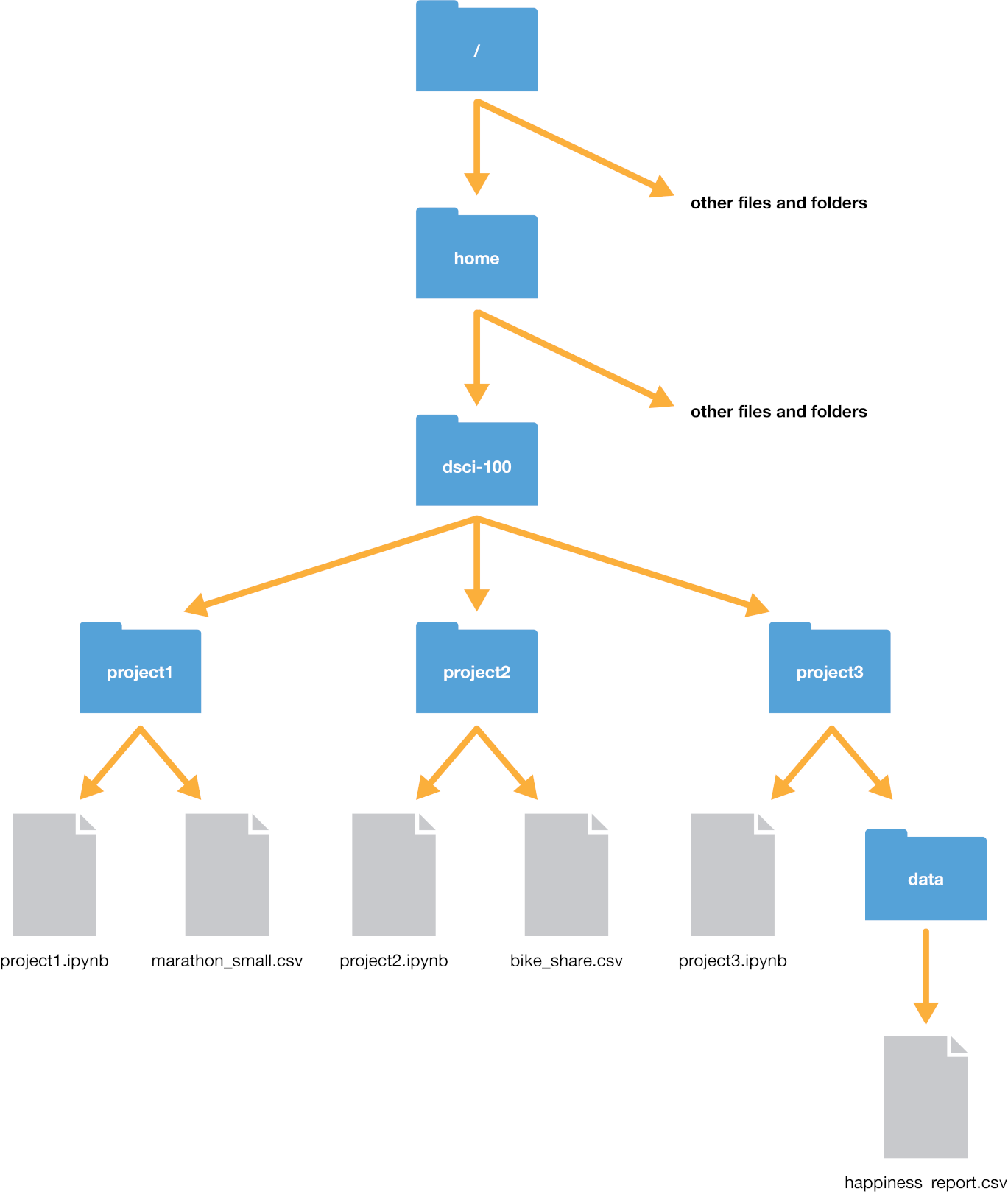
The place where your file lives is referred to as its ‘path’. You can think of the path as directions to the file. There are two kinds of paths:
- relative paths indicate where a file is with respect to your working directory
- absolute paths indicate where the file is with respect to the computers filesystem base (or root) folder, regardless of where you are working
Image from Data Science: A first introduction with Python (link)
In VSCode, your working directory is typically where your Jupyter notebook is saved.
import os
os.getcwd()'/Users/gm845/Library/CloudStorage/Box-Box/teaching/2025/msds-597/website/lec-2'We will be working with exchange rates data from the European Central Bank.
This data has the path:
/Users/gm845/Library/CloudStorage/Box-Box/teaching/2025/msds-597/lectures/data/rates.csvTo get to rates.csv, I need to “go one level up”, then enter the “data” folder.
Relative to the Jupyter notebook, this path is ../data/rates.csv. Here, ../ indicates “go one level up”.
df = pd.read_csv('../data/rates.csv')Note: the default is header=0 which takes the first row in the csv file as the column names.
Let’s look at the dataframe.
df.head() | Time | USD | JPY | BGN | CZK | DKK | GBP | CHF | |
|---|---|---|---|---|---|---|---|---|
| 0 | 2024-04-16 | 1.0637 | 164.54 | 1.9558 | 25.210 | 7.4609 | 0.85440 | 0.9712 |
| 1 | 2024-04-15 | 1.0656 | 164.05 | 1.9558 | 25.324 | 7.4606 | 0.85405 | 0.9725 |
| 2 | 2024-04-12 | 1.0652 | 163.16 | 1.9558 | 25.337 | 7.4603 | 0.85424 | 0.9716 |
| 3 | 2024-04-11 | 1.0729 | 164.18 | 1.9558 | 25.392 | 7.4604 | 0.85525 | 0.9787 |
| 4 | 2024-04-10 | 1.0860 | 164.89 | 1.9558 | 25.368 | 7.4594 | 0.85515 | 0.9810 |
df.tail()| Time | USD | JPY | BGN | CZK | DKK | GBP | CHF | |
|---|---|---|---|---|---|---|---|---|
| 57 | 2024-01-24 | 1.0905 | 160.46 | 1.9558 | 24.786 | 7.4568 | 0.85543 | 0.9415 |
| 58 | 2024-01-23 | 1.0872 | 160.88 | 1.9558 | 24.824 | 7.4574 | 0.85493 | 0.9446 |
| 59 | 2024-01-22 | 1.0890 | 160.95 | 1.9558 | 24.758 | 7.4585 | 0.85575 | 0.9458 |
| 60 | 2024-01-19 | 1.0887 | 161.17 | 1.9558 | 24.813 | 7.4575 | 0.85825 | 0.9459 |
| 61 | 2024-01-18 | 1.0875 | 160.89 | 1.9558 | 24.734 | 7.4571 | 0.85773 | 0.9432 |
df.shape(62, 8)We can inspect the data types of each column:
df.dtypesTime object
USD float64
JPY float64
BGN float64
CZK float64
DKK float64
GBP float64
CHF float64
dtype: objectWe see that the Time column has type object. We can fix this by reading in the data again, this time with the argument parse_dates=[`Time`]
df = pd.read_csv('../data/rates.csv', parse_dates=['Time'])
df.dtypes
Time datetime64[ns]
USD float64
JPY float64
BGN float64
CZK float64
DKK float64
GBP float64
CHF float64
dtype: objectAccessing a column
df['USD']0 1.0637
1 1.0656
2 1.0652
3 1.0729
4 1.0860
...
57 1.0905
58 1.0872
59 1.0890
60 1.0887
61 1.0875
Name: USD, Length: 62, dtype: float64isinstance(df['USD'], pd.Series)Truedf.USD0 1.0637
1 1.0656
2 1.0652
3 1.0729
4 1.0860
...
57 1.0905
58 1.0872
59 1.0890
60 1.0887
61 1.0875
Name: USD, Length: 62, dtype: float64Note: when we get the USD rates, we unfortunately lose information about the time.
# here is how to fix it and use time is index
df.index = df['Time']
df| Time | USD | JPY | BGN | CZK | DKK | GBP | CHF | |
|---|---|---|---|---|---|---|---|---|
| Time | ||||||||
| 2024-04-16 | 2024-04-16 | 1.0637 | 164.54 | 1.9558 | 25.210 | 7.4609 | 0.85440 | 0.9712 |
| 2024-04-15 | 2024-04-15 | 1.0656 | 164.05 | 1.9558 | 25.324 | 7.4606 | 0.85405 | 0.9725 |
| 2024-04-12 | 2024-04-12 | 1.0652 | 163.16 | 1.9558 | 25.337 | 7.4603 | 0.85424 | 0.9716 |
| 2024-04-11 | 2024-04-11 | 1.0729 | 164.18 | 1.9558 | 25.392 | 7.4604 | 0.85525 | 0.9787 |
| 2024-04-10 | 2024-04-10 | 1.0860 | 164.89 | 1.9558 | 25.368 | 7.4594 | 0.85515 | 0.9810 |
| ... | ... | ... | ... | ... | ... | ... | ... | ... |
| 2024-01-24 | 2024-01-24 | 1.0905 | 160.46 | 1.9558 | 24.786 | 7.4568 | 0.85543 | 0.9415 |
| 2024-01-23 | 2024-01-23 | 1.0872 | 160.88 | 1.9558 | 24.824 | 7.4574 | 0.85493 | 0.9446 |
| 2024-01-22 | 2024-01-22 | 1.0890 | 160.95 | 1.9558 | 24.758 | 7.4585 | 0.85575 | 0.9458 |
| 2024-01-19 | 2024-01-19 | 1.0887 | 161.17 | 1.9558 | 24.813 | 7.4575 | 0.85825 | 0.9459 |
| 2024-01-18 | 2024-01-18 | 1.0875 | 160.89 | 1.9558 | 24.734 | 7.4571 | 0.85773 | 0.9432 |
62 rows × 8 columns
# Now when we extract a column, we keep the index
# we keep information about the dates
df.USD
Time
2024-04-16 1.0637
2024-04-15 1.0656
2024-04-12 1.0652
2024-04-11 1.0729
2024-04-10 1.0860
...
2024-01-24 1.0905
2024-01-23 1.0872
2024-01-22 1.0890
2024-01-19 1.0887
2024-01-18 1.0875
Name: USD, Length: 62, dtype: float64Selecting/dropping multiple columns or rows
# Subsets of columns
df[['USD', 'CHF']]| USD | CHF | |
|---|---|---|
| Time | ||
| 2024-04-16 | 1.0637 | 0.9712 |
| 2024-04-15 | 1.0656 | 0.9725 |
| 2024-04-12 | 1.0652 | 0.9716 |
| 2024-04-11 | 1.0729 | 0.9787 |
| 2024-04-10 | 1.0860 | 0.9810 |
| ... | ... | ... |
| 2024-01-24 | 1.0905 | 0.9415 |
| 2024-01-23 | 1.0872 | 0.9446 |
| 2024-01-22 | 1.0890 | 0.9458 |
| 2024-01-19 | 1.0887 | 0.9459 |
| 2024-01-18 | 1.0875 | 0.9432 |
62 rows × 2 columns
df[['USD', 'CHF']].head()| USD | CHF | |
|---|---|---|
| Time | ||
| 2024-04-16 | 1.0637 | 0.9712 |
| 2024-04-15 | 1.0656 | 0.9725 |
| 2024-04-12 | 1.0652 | 0.9716 |
| 2024-04-11 | 1.0729 | 0.9787 |
| 2024-04-10 | 1.0860 | 0.9810 |
df
df_dropped = df.drop(columns=['Time', 'BGN', 'DKK', 'CZK'])
df_dropped.head()| USD | JPY | GBP | CHF | |
|---|---|---|---|---|
| Time | ||||
| 2024-04-16 | 1.0637 | 164.54 | 0.85440 | 0.9712 |
| 2024-04-15 | 1.0656 | 164.05 | 0.85405 | 0.9725 |
| 2024-04-12 | 1.0652 | 163.16 | 0.85424 | 0.9716 |
| 2024-04-11 | 1.0729 | 164.18 | 0.85525 | 0.9787 |
| 2024-04-10 | 1.0860 | 164.89 | 0.85515 | 0.9810 |
df.head() # original df unaffected| Time | USD | JPY | BGN | CZK | DKK | GBP | CHF | |
|---|---|---|---|---|---|---|---|---|
| Time | ||||||||
| 2024-04-16 | 2024-04-16 | 1.0637 | 164.54 | 1.9558 | 25.210 | 7.4609 | 0.85440 | 0.9712 |
| 2024-04-15 | 2024-04-15 | 1.0656 | 164.05 | 1.9558 | 25.324 | 7.4606 | 0.85405 | 0.9725 |
| 2024-04-12 | 2024-04-12 | 1.0652 | 163.16 | 1.9558 | 25.337 | 7.4603 | 0.85424 | 0.9716 |
| 2024-04-11 | 2024-04-11 | 1.0729 | 164.18 | 1.9558 | 25.392 | 7.4604 | 0.85525 | 0.9787 |
| 2024-04-10 | 2024-04-10 | 1.0860 | 164.89 | 1.9558 | 25.368 | 7.4594 | 0.85515 | 0.9810 |
# dropping a row
df_dropped.drop('2024-04-16').head()
# same as: df_dropped.drop(index='2024-04-16').head()| USD | JPY | GBP | CHF | |
|---|---|---|---|---|
| Time | ||||
| 2024-04-15 | 1.0656 | 164.05 | 0.85405 | 0.9725 |
| 2024-04-12 | 1.0652 | 163.16 | 0.85424 | 0.9716 |
| 2024-04-11 | 1.0729 | 164.18 | 0.85525 | 0.9787 |
| 2024-04-10 | 1.0860 | 164.89 | 0.85515 | 0.9810 |
| 2024-04-09 | 1.0867 | 164.97 | 0.85663 | 0.9819 |
# now that time is the index, let's drop the Time column
df = df.drop(columns='Time')
Selecting rows
Series
Note: be careful with accessing data - it will treat integers as labels
usd = df['USD'].copy()usd.index = [i * 2 for i in range(len(usd))]usd0 1.0637
2 1.0656
4 1.0652
6 1.0729
8 1.0860
...
114 1.0905
116 1.0872
118 1.0890
120 1.0887
122 1.0875
Name: USD, Length: 62, dtype: float64usd[2]np.float64(1.0656)To avoid this, use the .loc method for labels, and .iloc for integers.
usd.loc[2]np.float64(1.0656)usd.iloc[2]np.float64(1.0652)Dataframes
df.loc['2024-04-16']USD 1.0637
JPY 164.5400
BGN 1.9558
CZK 25.2100
DKK 7.4609
GBP 0.8544
CHF 0.9712
Name: 2024-04-16 00:00:00, dtype: float64df.loc['2024-04-16', ['USD', 'GBP']]USD 1.0637
GBP 0.8544
Name: 2024-04-16 00:00:00, dtype: float64df.loc[["2024-01-18"], ['USD', 'GBP']]| USD | GBP | |
|---|---|---|
| Time | ||
| 2024-01-18 | 1.0875 | 0.85773 |
print('First is', type(df.loc["2024-01-18", ['USD', 'GBP']]), ', second is', type(df.loc[["2024-01-18"], ['USD', 'GBP']]))First is <class 'pandas.core.series.Series'> , second is <class 'pandas.core.frame.DataFrame'>df.loc[["2024-01-18", "2024-04-16"], ['USD', 'GBP']]| USD | GBP | |
|---|---|---|
| Time | ||
| 2024-01-18 | 1.0875 | 0.85773 |
| 2024-04-16 | 1.0637 | 0.85440 |
# this will fail: df.loc[:, 1:3]
# loc expects labels for rows and columns
iloc
df.iloc[0]USD 1.0637
JPY 164.5400
BGN 1.9558
CZK 25.2100
DKK 7.4609
GBP 0.8544
CHF 0.9712
Name: 2024-04-16 00:00:00, dtype: float64df.iloc[:, 1:3]| JPY | BGN | |
|---|---|---|
| Time | ||
| 2024-04-16 | 164.54 | 1.9558 |
| 2024-04-15 | 164.05 | 1.9558 |
| 2024-04-12 | 163.16 | 1.9558 |
| 2024-04-11 | 164.18 | 1.9558 |
| 2024-04-10 | 164.89 | 1.9558 |
| ... | ... | ... |
| 2024-01-24 | 160.46 | 1.9558 |
| 2024-01-23 | 160.88 | 1.9558 |
| 2024-01-22 | 160.95 | 1.9558 |
| 2024-01-19 | 161.17 | 1.9558 |
| 2024-01-18 | 160.89 | 1.9558 |
62 rows × 2 columns
df.iloc[:, 1:] # all columns except 0th one| JPY | BGN | CZK | DKK | GBP | CHF | |
|---|---|---|---|---|---|---|
| Time | ||||||
| 2024-04-16 | 164.54 | 1.9558 | 25.210 | 7.4609 | 0.85440 | 0.9712 |
| 2024-04-15 | 164.05 | 1.9558 | 25.324 | 7.4606 | 0.85405 | 0.9725 |
| 2024-04-12 | 163.16 | 1.9558 | 25.337 | 7.4603 | 0.85424 | 0.9716 |
| 2024-04-11 | 164.18 | 1.9558 | 25.392 | 7.4604 | 0.85525 | 0.9787 |
| 2024-04-10 | 164.89 | 1.9558 | 25.368 | 7.4594 | 0.85515 | 0.9810 |
| ... | ... | ... | ... | ... | ... | ... |
| 2024-01-24 | 160.46 | 1.9558 | 24.786 | 7.4568 | 0.85543 | 0.9415 |
| 2024-01-23 | 160.88 | 1.9558 | 24.824 | 7.4574 | 0.85493 | 0.9446 |
| 2024-01-22 | 160.95 | 1.9558 | 24.758 | 7.4585 | 0.85575 | 0.9458 |
| 2024-01-19 | 161.17 | 1.9558 | 24.813 | 7.4575 | 0.85825 | 0.9459 |
| 2024-01-18 | 160.89 | 1.9558 | 24.734 | 7.4571 | 0.85773 | 0.9432 |
62 rows × 6 columns
df.iloc[:10, 1:4] # select a few rows, only keep columns 1,2,3| JPY | BGN | CZK | |
|---|---|---|---|
| Time | |||
| 2024-04-16 | 164.54 | 1.9558 | 25.210 |
| 2024-04-15 | 164.05 | 1.9558 | 25.324 |
| 2024-04-12 | 163.16 | 1.9558 | 25.337 |
| 2024-04-11 | 164.18 | 1.9558 | 25.392 |
| 2024-04-10 | 164.89 | 1.9558 | 25.368 |
| 2024-04-09 | 164.97 | 1.9558 | 25.380 |
| 2024-04-08 | 164.43 | 1.9558 | 25.354 |
| 2024-04-05 | 164.10 | 1.9558 | 25.286 |
| 2024-04-04 | 164.69 | 1.9558 | 25.322 |
| 2024-04-03 | 163.66 | 1.9558 | 25.352 |
| Type | Notes |
|---|---|
df[column] |
Select single column or sequence of columns from the DataFrame; special case conveniences: Boolean array (filter rows), slice (slice rows), or Boolean DataFrame (set values based on some criterion) |
df.loc[rows] |
Select single row or subset of rows from the DataFrame by label |
df.loc[:,cols] |
Select single column or subset of columns by label |
df.loc[rows,cols] |
Select both row(s) and column(s) by label |
df.iloc[rows] |
Select single row or subset of rows from the DataFrame by integer position |
df.iloc[:,cols] |
Select single column or subset of columns by integer position |
df.iloc[rows,cols] |
Select both row(s) and column(s) by integer position |
Selecting based on logical conditions
df.query('USD > 1.09')| USD | JPY | BGN | CZK | DKK | GBP | CHF | |
|---|---|---|---|---|---|---|---|
| Time | |||||||
| 2024-03-21 | 1.0907 | 164.96 | 1.9558 | 25.243 | 7.4579 | 0.85678 | 0.9766 |
| 2024-03-14 | 1.0925 | 161.70 | 1.9558 | 25.198 | 7.4568 | 0.85420 | 0.9616 |
| 2024-03-13 | 1.0939 | 161.83 | 1.9558 | 25.273 | 7.4573 | 0.85451 | 0.9599 |
| 2024-03-12 | 1.0916 | 161.39 | 1.9558 | 25.272 | 7.4571 | 0.85458 | 0.9588 |
| 2024-03-11 | 1.0926 | 160.43 | 1.9558 | 25.322 | 7.4552 | 0.85208 | 0.9594 |
| 2024-03-08 | 1.0932 | 160.99 | 1.9558 | 25.308 | 7.4547 | 0.85168 | 0.9588 |
| 2024-01-24 | 1.0905 | 160.46 | 1.9558 | 24.786 | 7.4568 | 0.85543 | 0.9415 |
df.query('USD > 1.09 and JPY < 161')| USD | JPY | BGN | CZK | DKK | GBP | CHF | |
|---|---|---|---|---|---|---|---|
| Time | |||||||
| 2024-03-11 | 1.0926 | 160.43 | 1.9558 | 25.322 | 7.4552 | 0.85208 | 0.9594 |
| 2024-03-08 | 1.0932 | 160.99 | 1.9558 | 25.308 | 7.4547 | 0.85168 | 0.9588 |
| 2024-01-24 | 1.0905 | 160.46 | 1.9558 | 24.786 | 7.4568 | 0.85543 | 0.9415 |
df.USD > 1.09 # boolean maskTime
2024-04-16 False
2024-04-15 False
2024-04-12 False
2024-04-11 False
2024-04-10 False
...
2024-01-24 True
2024-01-23 False
2024-01-22 False
2024-01-19 False
2024-01-18 False
Name: USD, Length: 62, dtype: booldf[df.USD > 1.09] # you can select boolean rows with []| USD | JPY | BGN | CZK | DKK | GBP | CHF | |
|---|---|---|---|---|---|---|---|
| Time | |||||||
| 2024-03-21 | 1.0907 | 164.96 | 1.9558 | 25.243 | 7.4579 | 0.85678 | 0.9766 |
| 2024-03-14 | 1.0925 | 161.70 | 1.9558 | 25.198 | 7.4568 | 0.85420 | 0.9616 |
| 2024-03-13 | 1.0939 | 161.83 | 1.9558 | 25.273 | 7.4573 | 0.85451 | 0.9599 |
| 2024-03-12 | 1.0916 | 161.39 | 1.9558 | 25.272 | 7.4571 | 0.85458 | 0.9588 |
| 2024-03-11 | 1.0926 | 160.43 | 1.9558 | 25.322 | 7.4552 | 0.85208 | 0.9594 |
| 2024-03-08 | 1.0932 | 160.99 | 1.9558 | 25.308 | 7.4547 | 0.85168 | 0.9588 |
| 2024-01-24 | 1.0905 | 160.46 | 1.9558 | 24.786 | 7.4568 | 0.85543 | 0.9415 |
mask1 = df.USD > 1.09
mask2 = df.JPY < 161
df[mask1 & mask2] # mask1 and mask2| USD | JPY | BGN | CZK | DKK | GBP | CHF | |
|---|---|---|---|---|---|---|---|
| Time | |||||||
| 2024-03-11 | 1.0926 | 160.43 | 1.9558 | 25.322 | 7.4552 | 0.85208 | 0.9594 |
| 2024-03-08 | 1.0932 | 160.99 | 1.9558 | 25.308 | 7.4547 | 0.85168 | 0.9588 |
| 2024-01-24 | 1.0905 | 160.46 | 1.9558 | 24.786 | 7.4568 | 0.85543 | 0.9415 |
df[mask1 | mask2].head() # mask1 or mask2| USD | JPY | BGN | CZK | DKK | GBP | CHF | |
|---|---|---|---|---|---|---|---|
| Time | |||||||
| 2024-03-21 | 1.0907 | 164.96 | 1.9558 | 25.243 | 7.4579 | 0.85678 | 0.9766 |
| 2024-03-14 | 1.0925 | 161.70 | 1.9558 | 25.198 | 7.4568 | 0.85420 | 0.9616 |
| 2024-03-13 | 1.0939 | 161.83 | 1.9558 | 25.273 | 7.4573 | 0.85451 | 0.9599 |
| 2024-03-12 | 1.0916 | 161.39 | 1.9558 | 25.272 | 7.4571 | 0.85458 | 0.9588 |
| 2024-03-11 | 1.0926 | 160.43 | 1.9558 | 25.322 | 7.4552 | 0.85208 | 0.9594 |
# this fails
# df[mask1 & mask2, 'USD']
# to select rows with booleans AND columns, use loc
Boolean arrays can be used with loc but not iloc:
df.loc[mask1 & mask2, 'USD']Time
2024-03-11 1.0926
2024-03-08 1.0932
2024-01-24 1.0905
Name: USD, dtype: float64# Using a boolean mask to select columns
df.columns != 'Time'array([ True, True, True, True, True, True, True])df_dropped2 = df.loc[:, df.columns != 'Time']
df_dropped2| USD | JPY | BGN | CZK | DKK | GBP | CHF | |
|---|---|---|---|---|---|---|---|
| Time | |||||||
| 2024-04-16 | 1.0637 | 164.54 | 1.9558 | 25.210 | 7.4609 | 0.85440 | 0.9712 |
| 2024-04-15 | 1.0656 | 164.05 | 1.9558 | 25.324 | 7.4606 | 0.85405 | 0.9725 |
| 2024-04-12 | 1.0652 | 163.16 | 1.9558 | 25.337 | 7.4603 | 0.85424 | 0.9716 |
| 2024-04-11 | 1.0729 | 164.18 | 1.9558 | 25.392 | 7.4604 | 0.85525 | 0.9787 |
| 2024-04-10 | 1.0860 | 164.89 | 1.9558 | 25.368 | 7.4594 | 0.85515 | 0.9810 |
| ... | ... | ... | ... | ... | ... | ... | ... |
| 2024-01-24 | 1.0905 | 160.46 | 1.9558 | 24.786 | 7.4568 | 0.85543 | 0.9415 |
| 2024-01-23 | 1.0872 | 160.88 | 1.9558 | 24.824 | 7.4574 | 0.85493 | 0.9446 |
| 2024-01-22 | 1.0890 | 160.95 | 1.9558 | 24.758 | 7.4585 | 0.85575 | 0.9458 |
| 2024-01-19 | 1.0887 | 161.17 | 1.9558 | 24.813 | 7.4575 | 0.85825 | 0.9459 |
| 2024-01-18 | 1.0875 | 160.89 | 1.9558 | 24.734 | 7.4571 | 0.85773 | 0.9432 |
62 rows × 7 columns
Sorting dataframes
df.sort_index()| USD | JPY | BGN | CZK | DKK | GBP | CHF | |
|---|---|---|---|---|---|---|---|
| Time | |||||||
| 2024-01-18 | 1.0875 | 160.89 | 1.9558 | 24.734 | 7.4571 | 0.85773 | 0.9432 |
| 2024-01-19 | 1.0887 | 161.17 | 1.9558 | 24.813 | 7.4575 | 0.85825 | 0.9459 |
| 2024-01-22 | 1.0890 | 160.95 | 1.9558 | 24.758 | 7.4585 | 0.85575 | 0.9458 |
| 2024-01-23 | 1.0872 | 160.88 | 1.9558 | 24.824 | 7.4574 | 0.85493 | 0.9446 |
| 2024-01-24 | 1.0905 | 160.46 | 1.9558 | 24.786 | 7.4568 | 0.85543 | 0.9415 |
| ... | ... | ... | ... | ... | ... | ... | ... |
| 2024-04-10 | 1.0860 | 164.89 | 1.9558 | 25.368 | 7.4594 | 0.85515 | 0.9810 |
| 2024-04-11 | 1.0729 | 164.18 | 1.9558 | 25.392 | 7.4604 | 0.85525 | 0.9787 |
| 2024-04-12 | 1.0652 | 163.16 | 1.9558 | 25.337 | 7.4603 | 0.85424 | 0.9716 |
| 2024-04-15 | 1.0656 | 164.05 | 1.9558 | 25.324 | 7.4606 | 0.85405 | 0.9725 |
| 2024-04-16 | 1.0637 | 164.54 | 1.9558 | 25.210 | 7.4609 | 0.85440 | 0.9712 |
62 rows × 7 columns
df.sort_index(axis='columns')| BGN | CHF | CZK | DKK | GBP | JPY | USD | |
|---|---|---|---|---|---|---|---|
| Time | |||||||
| 2024-04-16 | 1.9558 | 0.9712 | 25.210 | 7.4609 | 0.85440 | 164.54 | 1.0637 |
| 2024-04-15 | 1.9558 | 0.9725 | 25.324 | 7.4606 | 0.85405 | 164.05 | 1.0656 |
| 2024-04-12 | 1.9558 | 0.9716 | 25.337 | 7.4603 | 0.85424 | 163.16 | 1.0652 |
| 2024-04-11 | 1.9558 | 0.9787 | 25.392 | 7.4604 | 0.85525 | 164.18 | 1.0729 |
| 2024-04-10 | 1.9558 | 0.9810 | 25.368 | 7.4594 | 0.85515 | 164.89 | 1.0860 |
| ... | ... | ... | ... | ... | ... | ... | ... |
| 2024-01-24 | 1.9558 | 0.9415 | 24.786 | 7.4568 | 0.85543 | 160.46 | 1.0905 |
| 2024-01-23 | 1.9558 | 0.9446 | 24.824 | 7.4574 | 0.85493 | 160.88 | 1.0872 |
| 2024-01-22 | 1.9558 | 0.9458 | 24.758 | 7.4585 | 0.85575 | 160.95 | 1.0890 |
| 2024-01-19 | 1.9558 | 0.9459 | 24.813 | 7.4575 | 0.85825 | 161.17 | 1.0887 |
| 2024-01-18 | 1.9558 | 0.9432 | 24.734 | 7.4571 | 0.85773 | 160.89 | 1.0875 |
62 rows × 7 columns
df.USD.sort_values(ascending=False)Time
2024-03-13 1.0939
2024-03-08 1.0932
2024-03-11 1.0926
2024-03-14 1.0925
2024-03-12 1.0916
...
2024-04-11 1.0729
2024-02-14 1.0713
2024-04-15 1.0656
2024-04-12 1.0652
2024-04-16 1.0637
Name: USD, Length: 62, dtype: float64df_sorted = df.sort_values(by='USD', ascending=False)df_sorted.head()| USD | JPY | BGN | CZK | DKK | GBP | CHF | |
|---|---|---|---|---|---|---|---|
| Time | |||||||
| 2024-03-13 | 1.0939 | 161.83 | 1.9558 | 25.273 | 7.4573 | 0.85451 | 0.9599 |
| 2024-03-08 | 1.0932 | 160.99 | 1.9558 | 25.308 | 7.4547 | 0.85168 | 0.9588 |
| 2024-03-11 | 1.0926 | 160.43 | 1.9558 | 25.322 | 7.4552 | 0.85208 | 0.9594 |
| 2024-03-14 | 1.0925 | 161.70 | 1.9558 | 25.198 | 7.4568 | 0.85420 | 0.9616 |
| 2024-03-12 | 1.0916 | 161.39 | 1.9558 | 25.272 | 7.4571 | 0.85458 | 0.9588 |
Unique values
df.USD.unique()array([1.0637, 1.0656, 1.0652, 1.0729, 1.086 , 1.0867, 1.0823, 1.0841,
1.0852, 1.0783, 1.0749, 1.0811, 1.0816, 1.0855, 1.0835, 1.0907,
1.0844, 1.0854, 1.0892, 1.0925, 1.0939, 1.0916, 1.0926, 1.0932,
1.0895, 1.0874, 1.0849, 1.0846, 1.0813, 1.0826, 1.0808, 1.0856,
1.0834, 1.0809, 1.0802, 1.0776, 1.0768, 1.0743, 1.0713, 1.0793,
1.0773, 1.0772, 1.0758, 1.0746, 1.0883, 1.0814, 1.0837, 1.0871,
1.0893, 1.0905, 1.0872, 1.089 , 1.0887, 1.0875])df.USD.value_counts().head()USD
1.0823 3
1.0846 2
1.0844 2
1.0776 2
1.0852 2
Name: count, dtype: int64df.BGN.unique()array([1.9558])df.BGN.value_counts()BGN
1.9558 62
Name: count, dtype: int64Adding or modifying columns
df_copy = df.copy() # copy by value, not by referencedf_copy['new_col'] = 100 * df_copy.JPY/df_copy.USDdf_copy.head()| USD | JPY | BGN | CZK | DKK | GBP | CHF | new_col | |
|---|---|---|---|---|---|---|---|---|
| Time | ||||||||
| 2024-04-16 | 1.0637 | 164.54 | 1.9558 | 25.210 | 7.4609 | 0.85440 | 0.9712 | 15468.647175 |
| 2024-04-15 | 1.0656 | 164.05 | 1.9558 | 25.324 | 7.4606 | 0.85405 | 0.9725 | 15395.082583 |
| 2024-04-12 | 1.0652 | 163.16 | 1.9558 | 25.337 | 7.4603 | 0.85424 | 0.9716 | 15317.311303 |
| 2024-04-11 | 1.0729 | 164.18 | 1.9558 | 25.392 | 7.4604 | 0.85525 | 0.9787 | 15302.451300 |
| 2024-04-10 | 1.0860 | 164.89 | 1.9558 | 25.368 | 7.4594 | 0.85515 | 0.9810 | 15183.241252 |
df_copy[df_copy > 200] = 200# if we are changing a single column, use loc
df_copy.loc[df_copy['new_col'] == 200, 'new_col'] = 0df_copy| USD | JPY | BGN | CZK | DKK | GBP | CHF | new_col | |
|---|---|---|---|---|---|---|---|---|
| Time | ||||||||
| 2024-04-16 | 1.0637 | 164.54 | 1.9558 | 25.210 | 7.4609 | 0.85440 | 0.9712 | 0.0 |
| 2024-04-15 | 1.0656 | 164.05 | 1.9558 | 25.324 | 7.4606 | 0.85405 | 0.9725 | 0.0 |
| 2024-04-12 | 1.0652 | 163.16 | 1.9558 | 25.337 | 7.4603 | 0.85424 | 0.9716 | 0.0 |
| 2024-04-11 | 1.0729 | 164.18 | 1.9558 | 25.392 | 7.4604 | 0.85525 | 0.9787 | 0.0 |
| 2024-04-10 | 1.0860 | 164.89 | 1.9558 | 25.368 | 7.4594 | 0.85515 | 0.9810 | 0.0 |
| ... | ... | ... | ... | ... | ... | ... | ... | ... |
| 2024-01-24 | 1.0905 | 160.46 | 1.9558 | 24.786 | 7.4568 | 0.85543 | 0.9415 | 0.0 |
| 2024-01-23 | 1.0872 | 160.88 | 1.9558 | 24.824 | 7.4574 | 0.85493 | 0.9446 | 0.0 |
| 2024-01-22 | 1.0890 | 160.95 | 1.9558 | 24.758 | 7.4585 | 0.85575 | 0.9458 | 0.0 |
| 2024-01-19 | 1.0887 | 161.17 | 1.9558 | 24.813 | 7.4575 | 0.85825 | 0.9459 | 0.0 |
| 2024-01-18 | 1.0875 | 160.89 | 1.9558 | 24.734 | 7.4571 | 0.85773 | 0.9432 | 0.0 |
62 rows × 8 columns
Alternatively, we can use the assign function to create a new dataframe with the new column:
df.assign(new = df.USD/df.JPY * 100)| USD | JPY | BGN | CZK | DKK | GBP | CHF | new | |
|---|---|---|---|---|---|---|---|---|
| Time | ||||||||
| 2024-04-16 | 1.0637 | 164.54 | 1.9558 | 25.210 | 7.4609 | 0.85440 | 0.9712 | 0.646469 |
| 2024-04-15 | 1.0656 | 164.05 | 1.9558 | 25.324 | 7.4606 | 0.85405 | 0.9725 | 0.649558 |
| 2024-04-12 | 1.0652 | 163.16 | 1.9558 | 25.337 | 7.4603 | 0.85424 | 0.9716 | 0.652856 |
| 2024-04-11 | 1.0729 | 164.18 | 1.9558 | 25.392 | 7.4604 | 0.85525 | 0.9787 | 0.653490 |
| 2024-04-10 | 1.0860 | 164.89 | 1.9558 | 25.368 | 7.4594 | 0.85515 | 0.9810 | 0.658621 |
| ... | ... | ... | ... | ... | ... | ... | ... | ... |
| 2024-01-24 | 1.0905 | 160.46 | 1.9558 | 24.786 | 7.4568 | 0.85543 | 0.9415 | 0.679609 |
| 2024-01-23 | 1.0872 | 160.88 | 1.9558 | 24.824 | 7.4574 | 0.85493 | 0.9446 | 0.675783 |
| 2024-01-22 | 1.0890 | 160.95 | 1.9558 | 24.758 | 7.4585 | 0.85575 | 0.9458 | 0.676608 |
| 2024-01-19 | 1.0887 | 161.17 | 1.9558 | 24.813 | 7.4575 | 0.85825 | 0.9459 | 0.675498 |
| 2024-01-18 | 1.0875 | 160.89 | 1.9558 | 24.734 | 7.4571 | 0.85773 | 0.9432 | 0.675928 |
62 rows × 8 columns
df.head()| USD | JPY | BGN | CZK | DKK | GBP | CHF | |
|---|---|---|---|---|---|---|---|
| Time | |||||||
| 2024-04-16 | 1.0637 | 164.54 | 1.9558 | 25.210 | 7.4609 | 0.85440 | 0.9712 |
| 2024-04-15 | 1.0656 | 164.05 | 1.9558 | 25.324 | 7.4606 | 0.85405 | 0.9725 |
| 2024-04-12 | 1.0652 | 163.16 | 1.9558 | 25.337 | 7.4603 | 0.85424 | 0.9716 |
| 2024-04-11 | 1.0729 | 164.18 | 1.9558 | 25.392 | 7.4604 | 0.85525 | 0.9787 |
| 2024-04-10 | 1.0860 | 164.89 | 1.9558 | 25.368 | 7.4594 | 0.85515 | 0.9810 |
Concatenating
new_col = 100 * df_copy.JPY/df_copy.USDpd.concat([df_copy['USD'], new_col]) # vertical stackingTime
2024-04-16 1.063700
2024-04-15 1.065600
2024-04-12 1.065200
2024-04-11 1.072900
2024-04-10 1.086000
...
2024-01-24 14714.351215
2024-01-23 14797.645327
2024-01-22 14779.614325
2024-01-19 14803.894553
2024-01-18 14794.482759
Length: 124, dtype: float64pd.concat([df_copy['USD'], new_col], axis=1) # horizontal stacking| USD | 0 | |
|---|---|---|
| Time | ||
| 2024-04-16 | 1.0637 | 15468.647175 |
| 2024-04-15 | 1.0656 | 15395.082583 |
| 2024-04-12 | 1.0652 | 15317.311303 |
| 2024-04-11 | 1.0729 | 15302.451300 |
| 2024-04-10 | 1.0860 | 15183.241252 |
| ... | ... | ... |
| 2024-01-24 | 1.0905 | 14714.351215 |
| 2024-01-23 | 1.0872 | 14797.645327 |
| 2024-01-22 | 1.0890 | 14779.614325 |
| 2024-01-19 | 1.0887 | 14803.894553 |
| 2024-01-18 | 1.0875 | 14794.482759 |
62 rows × 2 columns
Summary statistics
Pandas objects have a set of common mathematical and statistical methods. Most of these fall into the category of reductions or summary statistics, methods that extract a single value (like the sum or mean) from a Series, or a Series of values from the rows or columns of a DataFrame. Pandas methods have built-in handling for missing data (unlike NumPy methods). Specifically, the default for pandas methods is skipna=True, which excludes NA/null values when computing the result.
df.mean()USD 1.082711
JPY 162.195484
BGN 1.955800
CZK 25.199081
DKK 7.456484
GBP 0.855201
CHF 0.957208
dtype: float64df_na = df.copy()df_na.iloc[0, 0] = np.nandf_na.head()| USD | JPY | BGN | CZK | DKK | GBP | CHF | |
|---|---|---|---|---|---|---|---|
| Time | |||||||
| 2024-04-16 | NaN | 164.54 | 1.9558 | 25.210 | 7.4609 | 0.85440 | 0.9712 |
| 2024-04-15 | 1.0656 | 164.05 | 1.9558 | 25.324 | 7.4606 | 0.85405 | 0.9725 |
| 2024-04-12 | 1.0652 | 163.16 | 1.9558 | 25.337 | 7.4603 | 0.85424 | 0.9716 |
| 2024-04-11 | 1.0729 | 164.18 | 1.9558 | 25.392 | 7.4604 | 0.85525 | 0.9787 |
| 2024-04-10 | 1.0860 | 164.89 | 1.9558 | 25.368 | 7.4594 | 0.85515 | 0.9810 |
df_na.mean()USD 1.083023
JPY 162.195484
BGN 1.955800
CZK 25.199081
DKK 7.456484
GBP 0.855201
CHF 0.957208
dtype: float64df_na.mean(skipna=False)USD NaN
JPY 162.195484
BGN 1.955800
CZK 25.199081
DKK 7.456484
GBP 0.855201
CHF 0.957208
dtype: float64df.describe()| USD | JPY | BGN | CZK | DKK | GBP | CHF | |
|---|---|---|---|---|---|---|---|
| count | 62.000000 | 62.000000 | 6.200000e+01 | 62.000000 | 62.000000 | 62.000000 | 62.000000 |
| mean | 1.082711 | 162.195484 | 1.955800e+00 | 25.199081 | 7.456484 | 0.855201 | 0.957208 |
| std | 0.006755 | 1.623635 | 2.686287e-15 | 0.220672 | 0.002161 | 0.001680 | 0.015174 |
| min | 1.063700 | 158.960000 | 1.955800e+00 | 24.734000 | 7.453600 | 0.850980 | 0.931500 |
| 25% | 1.078550 | 160.905000 | 1.955800e+00 | 25.046000 | 7.454425 | 0.854267 | 0.944900 |
| 50% | 1.083900 | 162.150000 | 1.955800e+00 | 25.297000 | 7.456500 | 0.855125 | 0.956150 |
| 75% | 1.087350 | 163.432500 | 1.955800e+00 | 25.354000 | 7.458200 | 0.856272 | 0.971500 |
| max | 1.093900 | 164.970000 | 1.955800e+00 | 25.460000 | 7.460900 | 0.858460 | 0.984600 |
df.describe(percentiles=[0.01, 0.05, 0.25, 0.75, 0.95])| USD | JPY | BGN | CZK | DKK | GBP | CHF | |
|---|---|---|---|---|---|---|---|
| count | 62.000000 | 62.000000 | 6.200000e+01 | 62.000000 | 62.000000 | 62.000000 | 62.000000 |
| mean | 1.082711 | 162.195484 | 1.955800e+00 | 25.199081 | 7.456484 | 0.855201 | 0.957208 |
| std | 0.006755 | 1.623635 | 2.686287e-15 | 0.220672 | 0.002161 | 0.001680 | 0.015174 |
| min | 1.063700 | 158.960000 | 1.955800e+00 | 24.734000 | 7.453600 | 0.850980 | 0.931500 |
| 1% | 1.064615 | 159.326000 | 1.955800e+00 | 24.742540 | 7.453661 | 0.851407 | 0.932781 |
| 5% | 1.071380 | 159.710500 | 1.955800e+00 | 24.759400 | 7.453905 | 0.852504 | 0.934705 |
| 25% | 1.078550 | 160.905000 | 1.955800e+00 | 25.046000 | 7.454425 | 0.854267 | 0.944900 |
| 50% | 1.083900 | 162.150000 | 1.955800e+00 | 25.297000 | 7.456500 | 0.855125 | 0.956150 |
| 75% | 1.087350 | 163.432500 | 1.955800e+00 | 25.354000 | 7.458200 | 0.856272 | 0.971500 |
| 95% | 1.092455 | 164.682500 | 1.955800e+00 | 25.414800 | 7.460395 | 0.857946 | 0.981000 |
| max | 1.093900 | 164.970000 | 1.955800e+00 | 25.460000 | 7.460900 | 0.858460 | 0.984600 |
df[['USD', 'CHF', 'CZK']].describe()| USD | CHF | CZK | |
|---|---|---|---|
| count | 62.000000 | 62.000000 | 62.000000 |
| mean | 1.082711 | 0.957208 | 25.199081 |
| std | 0.006755 | 0.015174 | 0.220672 |
| min | 1.063700 | 0.931500 | 24.734000 |
| 25% | 1.078550 | 0.944900 | 25.046000 |
| 50% | 1.083900 | 0.956150 | 25.297000 |
| 75% | 1.087350 | 0.971500 | 25.354000 |
| max | 1.093900 | 0.984600 | 25.460000 |
df.mean() USD 1.082711
JPY 162.195484
BGN 1.955800
CZK 25.199081
DKK 7.456484
GBP 0.855201
CHF 0.957208
dtype: float64df.median()USD 1.083900
JPY 162.150000
BGN 1.955800
CZK 25.297000
DKK 7.456500
GBP 0.855125
CHF 0.956150
dtype: float64df.min()USD 1.06370
JPY 158.96000
BGN 1.95580
CZK 24.73400
DKK 7.45360
GBP 0.85098
CHF 0.93150
dtype: float64type(df.mean())pandas.core.series.Seriesdf.agg(['mean', 'median']) # aggregate multiple statistics together| USD | JPY | BGN | CZK | DKK | GBP | CHF | |
|---|---|---|---|---|---|---|---|
| mean | 1.082711 | 162.195484 | 1.9558 | 25.199081 | 7.456484 | 0.855201 | 0.957208 |
| median | 1.083900 | 162.150000 | 1.9558 | 25.297000 | 7.456500 | 0.855125 | 0.956150 |
Correlation
df['USD'].corr(df['JPY'])np.float64(-0.10333665136813898)df.corr()| USD | JPY | BGN | CZK | DKK | GBP | CHF | |
|---|---|---|---|---|---|---|---|
| USD | 1.000000 | -0.103337 | NaN | -0.218888 | -0.232007 | 0.074199 | -0.042449 |
| JPY | -0.103337 | 1.000000 | NaN | 0.655093 | 0.463510 | 0.484794 | 0.901636 |
| BGN | NaN | NaN | NaN | NaN | NaN | NaN | NaN |
| CZK | -0.218888 | 0.655093 | NaN | 1.000000 | 0.008358 | 0.128065 | 0.649767 |
| DKK | -0.232007 | 0.463510 | NaN | 0.008358 | 1.000000 | 0.307508 | 0.604572 |
| GBP | 0.074199 | 0.484794 | NaN | 0.128065 | 0.307508 | 1.000000 | 0.424830 |
| CHF | -0.042449 | 0.901636 | NaN | 0.649767 | 0.604572 | 0.424830 | 1.000000 |
df.corrwith(df['USD'])USD 1.000000e+00
JPY -1.033367e-01
BGN -3.260316e-14
CZK -2.188876e-01
DKK -2.320074e-01
GBP 7.419901e-02
CHF -4.244863e-02
dtype: float64Operations between series
s1 = df['USD'].iloc[0:5].copy()
s1
Time
2024-04-16 1.0637
2024-04-15 1.0656
2024-04-12 1.0652
2024-04-11 1.0729
2024-04-10 1.0860
Name: USD, dtype: float64s2 = df['USD'].iloc[2:7].copy()
s2Time
2024-04-12 1.0652
2024-04-11 1.0729
2024-04-10 1.0860
2024-04-09 1.0867
2024-04-08 1.0823
Name: USD, dtype: float64s1 + s2Time
2024-04-08 NaN
2024-04-09 NaN
2024-04-10 2.1720
2024-04-11 2.1458
2024-04-12 2.1304
2024-04-15 NaN
2024-04-16 NaN
Freq: B, Name: USD, dtype: float64df1 = df.iloc[0:4, 0:3].copy()
df1| USD | JPY | BGN | |
|---|---|---|---|
| Time | |||
| 2024-04-16 | 1.0637 | 164.54 | 1.9558 |
| 2024-04-15 | 1.0656 | 164.05 | 1.9558 |
| 2024-04-12 | 1.0652 | 163.16 | 1.9558 |
| 2024-04-11 | 1.0729 | 164.18 | 1.9558 |
df2 = df.iloc[1:5, 1:4].copy()
df2| JPY | BGN | CZK | |
|---|---|---|---|
| Time | |||
| 2024-04-15 | 164.05 | 1.9558 | 25.324 |
| 2024-04-12 | 163.16 | 1.9558 | 25.337 |
| 2024-04-11 | 164.18 | 1.9558 | 25.392 |
| 2024-04-10 | 164.89 | 1.9558 | 25.368 |
df1 + df2| BGN | CZK | JPY | USD | |
|---|---|---|---|---|
| Time | ||||
| 2024-04-10 | NaN | NaN | NaN | NaN |
| 2024-04-11 | 3.9116 | NaN | 328.36 | NaN |
| 2024-04-12 | 3.9116 | NaN | 326.32 | NaN |
| 2024-04-15 | 3.9116 | NaN | 328.10 | NaN |
| 2024-04-16 | NaN | NaN | NaN | NaN |
When one dataframe is a subset of the other, you can do the following.
df1| USD | JPY | BGN | |
|---|---|---|---|
| Time | |||
| 2024-04-16 | 1.0637 | 164.54 | 1.9558 |
| 2024-04-15 | 1.0656 | 164.05 | 1.9558 |
| 2024-04-12 | 1.0652 | 163.16 | 1.9558 |
| 2024-04-11 | 1.0729 | 164.18 | 1.9558 |
df3 = df.iloc[0:3, 0:2].copy()
df3| USD | JPY | |
|---|---|---|
| Time | ||
| 2024-04-16 | 1.0637 | 164.54 |
| 2024-04-15 | 1.0656 | 164.05 |
| 2024-04-12 | 1.0652 | 163.16 |
df1.add(df3, fill_value=0)| BGN | JPY | USD | |
|---|---|---|---|
| Time | |||
| 2024-04-11 | 1.9558 | 164.18 | 1.0729 |
| 2024-04-12 | 1.9558 | 326.32 | 2.1304 |
| 2024-04-15 | 1.9558 | 328.10 | 2.1312 |
| 2024-04-16 | 1.9558 | 329.08 | 2.1274 |
Operations between dataframes and series
Operations between a dataframe and series follow similar broadcasting rules to numpy.
arr = np.arange(12.).reshape((3, 4))print(arr.shape, arr[0].shape) # trailing dimensions match(3, 4) (4,)arrarray([[ 0., 1., 2., 3.],
[ 4., 5., 6., 7.],
[ 8., 9., 10., 11.]])arr - arr[0]array([[0., 0., 0., 0.],
[4., 4., 4., 4.],
[8., 8., 8., 8.]])frame = pd.DataFrame(np.arange(12.).reshape((4, 3)), columns=list("bde"), index=["Utah", "Ohio", "Texas", "Oregon"])
series = frame.iloc[0]frame - series| b | d | e | |
|---|---|---|---|
| Utah | 0.0 | 0.0 | 0.0 |
| Ohio | 3.0 | 3.0 | 3.0 |
| Texas | 6.0 | 6.0 | 6.0 |
| Oregon | 9.0 | 9.0 | 9.0 |
series2 = pd.Series(np.arange(3), index=["b", "e", "f"])
frame + series2| b | d | e | f | |
|---|---|---|---|---|
| Utah | 0.0 | NaN | 3.0 | NaN |
| Ohio | 3.0 | NaN | 6.0 | NaN |
| Texas | 6.0 | NaN | 9.0 | NaN |
| Oregon | 9.0 | NaN | 12.0 | NaN |
If you want to instead broadcast over the columns, matching on the rows, you have to use one of the arithmetic methods and specify to match over the index. For example:
series3 = frame["d"]
series3
Utah 1.0
Ohio 4.0
Texas 7.0
Oregon 10.0
Name: d, dtype: float64frame.sub(series3, axis="index")| b | d | e | |
|---|---|---|---|
| Utah | -1.0 | 0.0 | 1.0 |
| Ohio | -1.0 | 0.0 | 1.0 |
| Texas | -1.0 | 0.0 | 1.0 |
| Oregon | -1.0 | 0.0 | 1.0 |
frame.sub(series3) # this doesn't do the right thing| Ohio | Oregon | Texas | Utah | b | d | e | |
|---|---|---|---|---|---|---|---|
| Utah | NaN | NaN | NaN | NaN | NaN | NaN | NaN |
| Ohio | NaN | NaN | NaN | NaN | NaN | NaN | NaN |
| Texas | NaN | NaN | NaN | NaN | NaN | NaN | NaN |
| Oregon | NaN | NaN | NaN | NaN | NaN | NaN | NaN |
Standardizing dataframes
df.mean()USD 1.082711
JPY 162.195484
BGN 1.955800
CZK 25.199081
DKK 7.456484
GBP 0.855201
CHF 0.957208
dtype: float64df - df.mean()| USD | JPY | BGN | CZK | DKK | GBP | CHF | |
|---|---|---|---|---|---|---|---|
| Time | |||||||
| 2024-04-16 | -0.019011 | 2.344516 | 4.440892e-16 | 0.010919 | 0.004416 | -0.000801 | 0.013992 |
| 2024-04-15 | -0.017111 | 1.854516 | 4.440892e-16 | 0.124919 | 0.004116 | -0.001151 | 0.015292 |
| 2024-04-12 | -0.017511 | 0.964516 | 4.440892e-16 | 0.137919 | 0.003816 | -0.000961 | 0.014392 |
| 2024-04-11 | -0.009811 | 1.984516 | 4.440892e-16 | 0.192919 | 0.003916 | 0.000049 | 0.021492 |
| 2024-04-10 | 0.003289 | 2.694516 | 4.440892e-16 | 0.168919 | 0.002916 | -0.000051 | 0.023792 |
| ... | ... | ... | ... | ... | ... | ... | ... |
| 2024-01-24 | 0.007789 | -1.735484 | 4.440892e-16 | -0.413081 | 0.000316 | 0.000229 | -0.015708 |
| 2024-01-23 | 0.004489 | -1.315484 | 4.440892e-16 | -0.375081 | 0.000916 | -0.000271 | -0.012608 |
| 2024-01-22 | 0.006289 | -1.245484 | 4.440892e-16 | -0.441081 | 0.002016 | 0.000549 | -0.011408 |
| 2024-01-19 | 0.005989 | -1.025484 | 4.440892e-16 | -0.386081 | 0.001016 | 0.003049 | -0.011308 |
| 2024-01-18 | 0.004789 | -1.305484 | 4.440892e-16 | -0.465081 | 0.000616 | 0.002529 | -0.014008 |
62 rows × 7 columns
df.sub(df.mean())| USD | JPY | BGN | CZK | DKK | GBP | CHF | |
|---|---|---|---|---|---|---|---|
| Time | |||||||
| 2024-04-16 | -0.019011 | 2.344516 | 4.440892e-16 | 0.010919 | 0.004416 | -0.000801 | 0.013992 |
| 2024-04-15 | -0.017111 | 1.854516 | 4.440892e-16 | 0.124919 | 0.004116 | -0.001151 | 0.015292 |
| 2024-04-12 | -0.017511 | 0.964516 | 4.440892e-16 | 0.137919 | 0.003816 | -0.000961 | 0.014392 |
| 2024-04-11 | -0.009811 | 1.984516 | 4.440892e-16 | 0.192919 | 0.003916 | 0.000049 | 0.021492 |
| 2024-04-10 | 0.003289 | 2.694516 | 4.440892e-16 | 0.168919 | 0.002916 | -0.000051 | 0.023792 |
| ... | ... | ... | ... | ... | ... | ... | ... |
| 2024-01-24 | 0.007789 | -1.735484 | 4.440892e-16 | -0.413081 | 0.000316 | 0.000229 | -0.015708 |
| 2024-01-23 | 0.004489 | -1.315484 | 4.440892e-16 | -0.375081 | 0.000916 | -0.000271 | -0.012608 |
| 2024-01-22 | 0.006289 | -1.245484 | 4.440892e-16 | -0.441081 | 0.002016 | 0.000549 | -0.011408 |
| 2024-01-19 | 0.005989 | -1.025484 | 4.440892e-16 | -0.386081 | 0.001016 | 0.003049 | -0.011308 |
| 2024-01-18 | 0.004789 | -1.305484 | 4.440892e-16 | -0.465081 | 0.000616 | 0.002529 | -0.014008 |
62 rows × 7 columns
df.sub(df.mean()).mean() # almost zero: successUSD -2.184632e-16
JPY 3.483951e-14
BGN 4.440892e-16
CZK -5.042561e-15
DKK -9.311548e-16
GBP 1.146037e-16
CHF -2.148819e-17
dtype: float64df.sub(df.mean(), axis="columns")| USD | JPY | BGN | CZK | DKK | GBP | CHF | |
|---|---|---|---|---|---|---|---|
| Time | |||||||
| 2024-04-16 | -0.019011 | 2.344516 | 4.440892e-16 | 0.010919 | 0.004416 | -0.000801 | 0.013992 |
| 2024-04-15 | -0.017111 | 1.854516 | 4.440892e-16 | 0.124919 | 0.004116 | -0.001151 | 0.015292 |
| 2024-04-12 | -0.017511 | 0.964516 | 4.440892e-16 | 0.137919 | 0.003816 | -0.000961 | 0.014392 |
| 2024-04-11 | -0.009811 | 1.984516 | 4.440892e-16 | 0.192919 | 0.003916 | 0.000049 | 0.021492 |
| 2024-04-10 | 0.003289 | 2.694516 | 4.440892e-16 | 0.168919 | 0.002916 | -0.000051 | 0.023792 |
| ... | ... | ... | ... | ... | ... | ... | ... |
| 2024-01-24 | 0.007789 | -1.735484 | 4.440892e-16 | -0.413081 | 0.000316 | 0.000229 | -0.015708 |
| 2024-01-23 | 0.004489 | -1.315484 | 4.440892e-16 | -0.375081 | 0.000916 | -0.000271 | -0.012608 |
| 2024-01-22 | 0.006289 | -1.245484 | 4.440892e-16 | -0.441081 | 0.002016 | 0.000549 | -0.011408 |
| 2024-01-19 | 0.005989 | -1.025484 | 4.440892e-16 | -0.386081 | 0.001016 | 0.003049 | -0.011308 |
| 2024-01-18 | 0.004789 | -1.305484 | 4.440892e-16 | -0.465081 | 0.000616 | 0.002529 | -0.014008 |
62 rows × 7 columns
# also works, but maybe less explicit than axis="columns"
df.sub(df.mean(), axis=1).mean()
USD -2.184632e-16
JPY 3.483951e-14
BGN 4.440892e-16
CZK -5.042561e-15
DKK -9.311548e-16
GBP 1.146037e-16
CHF -2.148819e-17
dtype: float64df_standardized = (df-df.mean())/df.std()df_standardized2 = df.sub(df.mean()).div(df.std())# most explicit
df_standardized3 = df.sub(df.mean(), axis="columns").div(df.std(), axis="columns")df_standardized4 = df.sub(df.mean(), axis=1).div(df.std(), axis=1)((df_standardized4-df_standardized) == 0.).all()USD True
JPY True
BGN True
CZK True
DKK True
GBP True
CHF True
dtype: booldf_max_standardized = df/df.max()df_standardized| USD | JPY | BGN | CZK | DKK | GBP | CHF | |
|---|---|---|---|---|---|---|---|
| Time | |||||||
| 2024-04-16 | -2.814246 | 1.443993 | 0.165317 | 0.049482 | 2.043993 | -0.476651 | 0.922100 |
| 2024-04-15 | -2.532988 | 1.142200 | 0.165317 | 0.566086 | 1.905139 | -0.684975 | 1.007773 |
| 2024-04-12 | -2.592200 | 0.594048 | 0.165317 | 0.624997 | 1.766285 | -0.571885 | 0.948461 |
| 2024-04-11 | -1.452368 | 1.222268 | 0.165317 | 0.874235 | 1.812570 | 0.029281 | 1.416367 |
| 2024-04-10 | 0.486828 | 1.659558 | 0.165317 | 0.765476 | 1.349722 | -0.030241 | 1.567942 |
| ... | ... | ... | ... | ... | ... | ... | ... |
| 2024-01-24 | 1.152964 | -1.068888 | 0.165317 | -1.871920 | 0.146319 | 0.136419 | -1.035197 |
| 2024-01-23 | 0.664465 | -0.810209 | 0.165317 | -1.699719 | 0.424028 | -0.161188 | -0.830900 |
| 2024-01-22 | 0.930919 | -0.767096 | 0.165317 | -1.998805 | 0.933160 | 0.326887 | -0.751817 |
| 2024-01-19 | 0.886510 | -0.631598 | 0.165317 | -1.749567 | 0.470313 | 1.814921 | -0.745227 |
| 2024-01-18 | 0.708874 | -0.804050 | 0.165317 | -2.107564 | 0.285174 | 1.505410 | -0.923163 |
62 rows × 7 columns
Function application and mapping
def f1(x):
return x.max() - x.min()df.apply(f1) # applies across rows by defaultUSD 0.03020
JPY 6.01000
BGN 0.00000
CZK 0.72600
DKK 0.00730
GBP 0.00748
CHF 0.05310
dtype: float64df.apply(f1, axis='columns')Time
2024-04-16 163.68560
2024-04-15 163.19595
2024-04-12 162.30576
2024-04-11 163.32475
2024-04-10 164.03485
...
2024-01-24 159.60457
2024-01-23 160.02507
2024-01-22 160.09425
2024-01-19 160.31175
2024-01-18 160.03227
Length: 62, dtype: float64def f2(x):
return pd.Series([x.min(), x.max()], index=["min", "max"])df.apply(f2)| USD | JPY | BGN | CZK | DKK | GBP | CHF | |
|---|---|---|---|---|---|---|---|
| min | 1.0637 | 158.96 | 1.9558 | 24.734 | 7.4536 | 0.85098 | 0.9315 |
| max | 1.0939 | 164.97 | 1.9558 | 25.460 | 7.4609 | 0.85846 | 0.9846 |
def my_format(x):
    return f"{x:.2f}"
For element-wise operations, use pd.DataFrame.map:
df.map(my_format) | USD | JPY | BGN | CZK | DKK | GBP | CHF | |
|---|---|---|---|---|---|---|---|
| Time | |||||||
| 2024-04-16 | 1.06 | 164.54 | 1.96 | 25.21 | 7.46 | 0.85 | 0.97 |
| 2024-04-15 | 1.07 | 164.05 | 1.96 | 25.32 | 7.46 | 0.85 | 0.97 |
| 2024-04-12 | 1.07 | 163.16 | 1.96 | 25.34 | 7.46 | 0.85 | 0.97 |
| 2024-04-11 | 1.07 | 164.18 | 1.96 | 25.39 | 7.46 | 0.86 | 0.98 |
| 2024-04-10 | 1.09 | 164.89 | 1.96 | 25.37 | 7.46 | 0.86 | 0.98 |
| ... | ... | ... | ... | ... | ... | ... | ... |
| 2024-01-24 | 1.09 | 160.46 | 1.96 | 24.79 | 7.46 | 0.86 | 0.94 |
| 2024-01-23 | 1.09 | 160.88 | 1.96 | 24.82 | 7.46 | 0.85 | 0.94 |
| 2024-01-22 | 1.09 | 160.95 | 1.96 | 24.76 | 7.46 | 0.86 | 0.95 |
| 2024-01-19 | 1.09 | 161.17 | 1.96 | 24.81 | 7.46 | 0.86 | 0.95 |
| 2024-01-18 | 1.09 | 160.89 | 1.96 | 24.73 | 7.46 | 0.86 | 0.94 |
62 rows × 7 columns
df.map(lambda x: f"{x:.2f}")| USD | JPY | BGN | CZK | DKK | GBP | CHF | |
|---|---|---|---|---|---|---|---|
| Time | |||||||
| 2024-04-16 | 1.06 | 164.54 | 1.96 | 25.21 | 7.46 | 0.85 | 0.97 |
| 2024-04-15 | 1.07 | 164.05 | 1.96 | 25.32 | 7.46 | 0.85 | 0.97 |
| 2024-04-12 | 1.07 | 163.16 | 1.96 | 25.34 | 7.46 | 0.85 | 0.97 |
| 2024-04-11 | 1.07 | 164.18 | 1.96 | 25.39 | 7.46 | 0.86 | 0.98 |
| 2024-04-10 | 1.09 | 164.89 | 1.96 | 25.37 | 7.46 | 0.86 | 0.98 |
| ... | ... | ... | ... | ... | ... | ... | ... |
| 2024-01-24 | 1.09 | 160.46 | 1.96 | 24.79 | 7.46 | 0.86 | 0.94 |
| 2024-01-23 | 1.09 | 160.88 | 1.96 | 24.82 | 7.46 | 0.85 | 0.94 |
| 2024-01-22 | 1.09 | 160.95 | 1.96 | 24.76 | 7.46 | 0.86 | 0.95 |
| 2024-01-19 | 1.09 | 161.17 | 1.96 | 24.81 | 7.46 | 0.86 | 0.95 |
| 2024-01-18 | 1.09 | 160.89 | 1.96 | 24.73 | 7.46 | 0.86 | 0.94 |
62 rows × 7 columns
Wide vs. long data formats
df_standardized = df_standardized.reset_index() # turn time back into a columndf_standardized.head()| Time | USD | JPY | BGN | CZK | DKK | GBP | CHF | |
|---|---|---|---|---|---|---|---|---|
| 0 | 2024-04-16 | -2.814246 | 1.443993 | 0.165317 | 0.049482 | 2.043993 | -0.476651 | 0.922100 |
| 1 | 2024-04-15 | -2.532988 | 1.142200 | 0.165317 | 0.566086 | 1.905139 | -0.684975 | 1.007773 |
| 2 | 2024-04-12 | -2.592200 | 0.594048 | 0.165317 | 0.624997 | 1.766285 | -0.571885 | 0.948461 |
| 3 | 2024-04-11 | -1.452368 | 1.222268 | 0.165317 | 0.874235 | 1.812570 | 0.029281 | 1.416367 |
| 4 | 2024-04-10 | 0.486828 | 1.659558 | 0.165317 | 0.765476 | 1.349722 | -0.030241 | 1.567942 |
The data is in what’s known as a ‘wide’ format. This is because the currency is in each of the columns. We can transform it to a ‘long’ format by using melt with arguments:
id_vars: this is the column to be used as identifier variablesvar_name: this is the new column which will contain the names of the columns in wide formatvalue_name: this is the new column which will contain the values of the columns in wide format
df_long = df_standardized.melt(id_vars='Time', var_name='currency', value_name='rate')df_long| Time | currency | rate | |
|---|---|---|---|
| 0 | 2024-04-16 | USD | -2.814246 |
| 1 | 2024-04-15 | USD | -2.532988 |
| 2 | 2024-04-12 | USD | -2.592200 |
| 3 | 2024-04-11 | USD | -1.452368 |
| 4 | 2024-04-10 | USD | 0.486828 |
| ... | ... | ... | ... |
| 429 | 2024-01-24 | CHF | -1.035197 |
| 430 | 2024-01-23 | CHF | -0.830900 |
| 431 | 2024-01-22 | CHF | -0.751817 |
| 432 | 2024-01-19 | CHF | -0.745227 |
| 433 | 2024-01-18 | CHF | -0.923163 |
434 rows × 3 columns
This “long’ format is an example of a”tidy data frame”, which we will discuss in more detail next lecture.
To go back to the “wide” format, we can use the pivot method:
df_long.pivot(index=['Time'], # column which will be the index
              columns=['currency'], # variable which will expand out to columns
values=['rate']) # values in the table| rate | |||||||
|---|---|---|---|---|---|---|---|
| currency | BGN | CHF | CZK | DKK | GBP | JPY | USD |
| Time | |||||||
| 2024-01-18 | 0.165317 | -0.923163 | -2.107564 | 0.285174 | 1.505410 | -0.804050 | 0.708874 |
| 2024-01-19 | 0.165317 | -0.745227 | -1.749567 | 0.470313 | 1.814921 | -0.631598 | 0.886510 |
| 2024-01-22 | 0.165317 | -0.751817 | -1.998805 | 0.933160 | 0.326887 | -0.767096 | 0.930919 |
| 2024-01-23 | 0.165317 | -0.830900 | -1.699719 | 0.424028 | -0.161188 | -0.810209 | 0.664465 |
| 2024-01-24 | 0.165317 | -1.035197 | -1.871920 | 0.146319 | 0.136419 | -1.068888 | 1.152964 |
| ... | ... | ... | ... | ... | ... | ... | ... |
| 2024-04-10 | 0.165317 | 1.567942 | 0.765476 | 1.349722 | -0.030241 | 1.659558 | 0.486828 |
| 2024-04-11 | 0.165317 | 1.416367 | 0.874235 | 1.812570 | 0.029281 | 1.222268 | -1.452368 |
| 2024-04-12 | 0.165317 | 0.948461 | 0.624997 | 1.766285 | -0.571885 | 0.594048 | -2.592200 |
| 2024-04-15 | 0.165317 | 1.007773 | 0.566086 | 1.905139 | -0.684975 | 1.142200 | -2.532988 |
| 2024-04-16 | 0.165317 | 0.922100 | 0.049482 | 2.043993 | -0.476651 | 1.443993 | -2.814246 |
62 rows × 7 columns
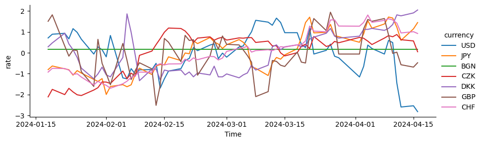
Example visualization with seaborn
We use the “long” data for a Seaborn plot:
sns.relplot(data=df_long,
            x='Time',
            y='rate',
            hue='currency',
            kind='line',
            height=3,
            aspect=3)