Lecture 5b - Variable Selection

Subset selection methods

Adapted from Introduction to Statistical Learning with Python (link)

Here we implement methods that reduce the number of parameters in a model by restricting the model to a subset of the input variables.

Forward Selection

We will apply the forward-selection approach to the Hitters data. We wish to predict a baseball player’s Salary on the basis of various statistics associated with performance in the previous year.

import numpy as np
import pandas as pd
import matplotlib.pyplot as plt
from matplotlib.pyplot import subplots
from statsmodels.api import OLS
import sklearn.linear_model as skl
from sklearn.preprocessing import StandardScaler
from ISLP import load_data
from ISLP.models import ModelSpec as MS
from sklearn.pipeline import Pipeline
from matplotlib.ticker import MaxNLocator
import warnings
warnings.simplefilter("ignore")

Hitters = load_data('Hitters')
Hitters = Hitters.dropna(); # remove rows with one or more missing values
Hitters.shape

(263, 20)

X = MS(Hitters.columns.drop('Salary')).fit_transform(Hitters)
Y = np.array(Hitters['Salary'])
sigma2 = OLS(Y,X).fit().scale

def Cp(sigma2, estimator, X, Y):
    "Cp statistic"
    n, p = X.shape
    Yhat = estimator.predict(X)
    RSS = np.sum((Y - Yhat)**2)
    return (RSS + 2 * p * sigma2) / n 

def RSS(estimator, X, Y):
    Yhat = estimator.predict(X)
    RSS = np.sum((Y - Yhat)**2)
    return RSS

# Forward stepwise

n = len(Y)
predictors = X.columns.drop('intercept')

selected = ['intercept']
remaining = predictors.copy()
variable_path = []
cp_path = []
rss_path = []

# include intercept-only model
X_current = X[selected]
fit0 = OLS(Y, X_current).fit()
cp0 = Cp(sigma2, fit0, X_current, Y)
rss0 = RSS(fit0, X_current, Y)
variable_path.append({"predictors": selected.copy()})
cp_path.append(cp0)
rss_path.append(rss0)

# build up models
for j in range(len(predictors)):
    best = None
    for cand in remaining:
        trial = selected + [cand]
        fit = OLS(Y, X[trial]).fit()
        cp = Cp(sigma2, fit, X[trial], Y)
        rss = RSS(fit, X[trial], Y)
        if (best is None) or (cp < best["cp"]):
            best = {"cand": cand, "cp": cp, "rss": rss}

    selected.append(best["cand"])
    remaining = remaining.drop(best["cand"])

    p = len(selected)
    variable_path.append({"predictors": selected.copy()})
    cp_path.append(best['cp'])
    rss_path.append(best['rss'])

np.argmin(cp_path)

np.int64(10)

variable_path[np.argmin(cp_path)]

{'predictors': ['intercept',
  'CRBI',
  'Hits',
  'PutOuts',
  'Division[W]',
  'AtBat',
  'Walks',
  'CWalks',
  'CRuns',
  'CAtBat',
  'Assists']}

fig, axs = plt.subplots(1, 2, figsize=(10, 4))

# Cp on left
axs[0].plot(cp_path, marker='o')
axs[0].set_xlabel('Step')
axs[0].set_ylabel('Cp')
axs[0].set_title('Cp path')
axs[0].grid(True)
axs[0].xaxis.set_major_locator(MaxNLocator(integer=True))

# RSS on right
axs[1].plot(rss_path, marker='s', color='orange')
axs[1].set_xlabel('Step')
axs[1].set_ylabel('RSS')
axs[1].set_title('RSS path')
axs[1].grid(True)
axs[1].xaxis.set_major_locator(MaxNLocator(integer=True))

plt.tight_layout()
plt.show()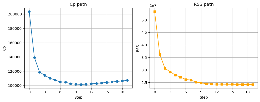

Backward stepwise

n = len(Y)
predictors = X.columns.drop('intercept')

selected = predictors.copy()
variable_path = []
cp_path = []
rss_path = []

fit = OLS(Y, X).fit()
cp = Cp(sigma2, fit, X, Y)
rss = RSS(fit, X, Y)
variable_path.append({"predictors": selected.copy()})
cp_path.append(cp)
rss_path.append(rss)

for j in range(len(predictors)):
    best = None
    for cand in selected:
        trial = [p for p in selected if p != cand]
        trial_all = ['intercept'] + trial
        fit = OLS(Y, X[trial_all]).fit()
        cp = Cp(sigma2, fit, X[trial_all], Y)
        rss = RSS(fit, X[trial_all], Y)
        if (best is None) or (cp < best["cp"]):
            best = {"rm": cand, "cp": cp, "rss": rss, "trial": trial}

    selected = best['trial']

    variable_path.append({"predictors": selected.copy()})
    cp_path.append(best['cp'])
    rss_path.append(best['rss'])

variable_path[np.argmin(cp_path)]

{'predictors': ['AtBat',
  'Hits',
  'Walks',
  'CAtBat',
  'CRuns',
  'CRBI',
  'CWalks',
  'Division[W]',
  'PutOuts',
  'Assists']}

fig, axs = plt.subplots(1, 2, figsize=(10, 4))

# Cp on left
axs[0].plot(np.arange(0, p)[::-1], cp_path, marker='o')
axs[0].set_xlabel('Step')
axs[0].set_ylabel('Cp')
axs[0].set_title('Cp path')
axs[0].grid(True)
axs[0].xaxis.set_major_locator(MaxNLocator(integer=True))

# RSS on right
axs[1].plot(np.arange(0, p)[::-1],rss_path, marker='s', color='orange')
axs[1].set_xlabel('Step')
axs[1].set_ylabel('RSS')
axs[1].set_title('RSS path')
axs[1].grid(True)
axs[1].xaxis.set_major_locator(MaxNLocator(integer=True))

plt.tight_layout()
plt.show()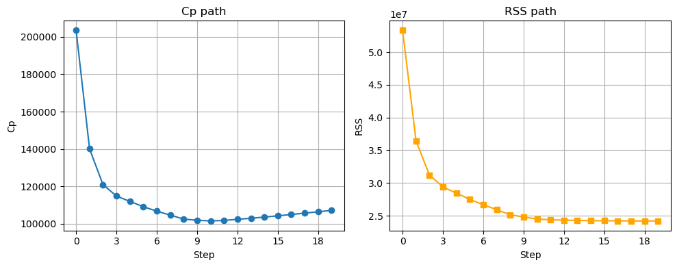

We get the same answer, whether we do forward or backward stepwise!

The Lasso

We now fit the Lasso. We use K-fold cross-validation to select the regularization parameter, \lambda.

K=5
scaler = StandardScaler(with_mean=True, with_std=True)

dat = MS(Hitters.columns.drop('Salary')).fit_transform(Hitters)
dat = dat.drop('intercept', axis=1) # remove intercept - it is added automatically
X = np.asarray(dat)

We use Pipeline to pipe together the standardization step and the lassoCV step.

lassoCV = skl.ElasticNetCV(alphas=100, # search over 100 different values of lambda
                           l1_ratio=1,
                           cv=K)
pipeCV = Pipeline(steps=[('scaler', scaler),
                         ('lasso', lassoCV)])
pipeCV.fit(X, Y)
tuned_lasso = pipeCV.named_steps['lasso']

lassoCV runs cross-validation for the following candidate \lambda values (determined automatically):

tuned_lasso.alphas_

array([255.28209651, 238.0769376 , 222.03134882, 207.06717903,
       193.11154419, 180.09647243, 167.95857295, 156.63872727,
       146.08180131, 136.23637682, 127.05450099, 118.49145286,
       110.50552551, 103.05782294,  96.1120706 ,  89.63443871,
        83.59337754,  77.95946367,  72.70525674,  67.80516577,
        63.23532454,  58.9734753 ,  54.99886045,  51.29212133,
        47.83520402,  44.61127137,  41.60462098,  38.80060878,
        36.18557761,  33.74679078,  31.47237003,  29.35123763,
        27.37306245,  25.52820965,  23.80769376,  22.20313488,
        20.7067179 ,  19.31115442,  18.00964724,  16.7958573 ,
        15.66387273,  14.60818013,  13.62363768,  12.7054501 ,
        11.84914529,  11.05055255,  10.30578229,   9.61120706,
         8.96344387,   8.35933775,   7.79594637,   7.27052567,
         6.78051658,   6.32353245,   5.89734753,   5.49988604,
         5.12921213,   4.7835204 ,   4.46112714,   4.1604621 ,
         3.88006088,   3.61855776,   3.37467908,   3.147237  ,
         2.93512376,   2.73730624,   2.55282097,   2.38076938,
         2.22031349,   2.07067179,   1.93111544,   1.80096472,
         1.67958573,   1.56638727,   1.46081801,   1.36236377,
         1.27054501,   1.18491453,   1.10505526,   1.03057823,
         0.96112071,   0.89634439,   0.83593378,   0.77959464,
         0.72705257,   0.67805166,   0.63235325,   0.58973475,
         0.5499886 ,   0.51292121,   0.47835204,   0.44611271,
         0.41604621,   0.38800609,   0.36185578,   0.33746791,
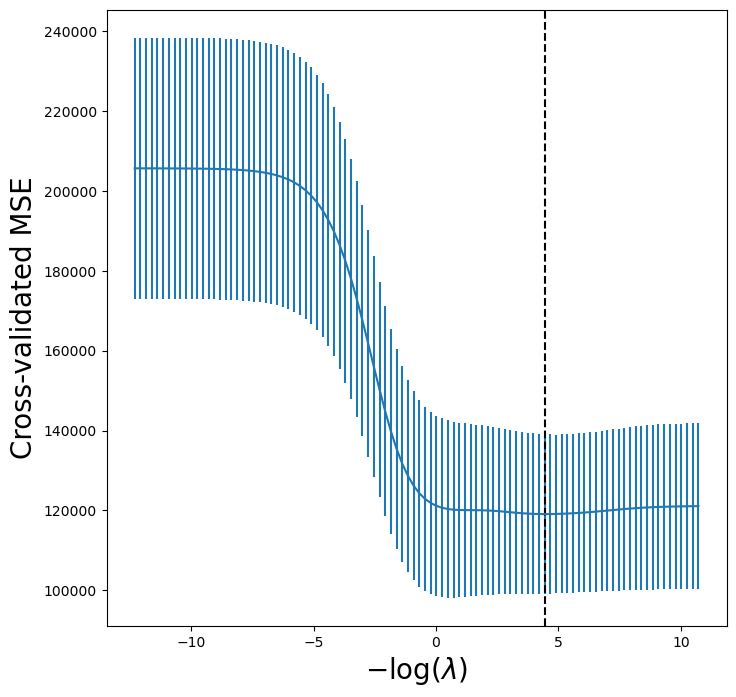
         0.3147237 ,   0.29351238,   0.27373062,   0.2552821 ])

The \lambda with lowest CV error is:

tuned_lasso.alpha_

np.float64(2.737306244504529)

The corresponding coefficients are:

tuned_lasso.coef_

array([-226.83004696,  254.82706494,    0.        ,   -0.        ,
          0.        ,  102.14493902,  -44.59414305,   -0.        ,
          0.        ,   43.36295623,  218.02899432,  123.42086296,
       -138.61718612,   16.04104388,  -59.54521107,   76.10379606,
         24.74415012,  -13.25252655,   -0.        ])

LassoCV doesn’t store all the coefficients for each \lambda candidate. To visualize the Lasso paths, let’s obtain these coefficients for every \lambda:

scale = pipeCV.named_steps['scaler']
Xs = scale.transform(X)

lambdas, soln_array = skl.Lasso.path(Xs, 
                                    Y,
                                    l1_ratio=1,
                                    n_alphas=100)[:2]
soln_path = pd.DataFrame(soln_array.T,
                         columns=dat.columns,
                         index=-np.log(lambdas))

path_fig, ax = subplots(figsize=(8,8))
soln_path.plot(ax=ax, legend=False)
ax.legend(loc='upper left')
ax.set_xlabel('$-\\log(\\lambda)$', fontsize=20)
ax.set_ylabel('Standardized coefficients', fontsize=20);
ax.axvline(-np.log(tuned_lasso.alpha_), c='k', ls='--')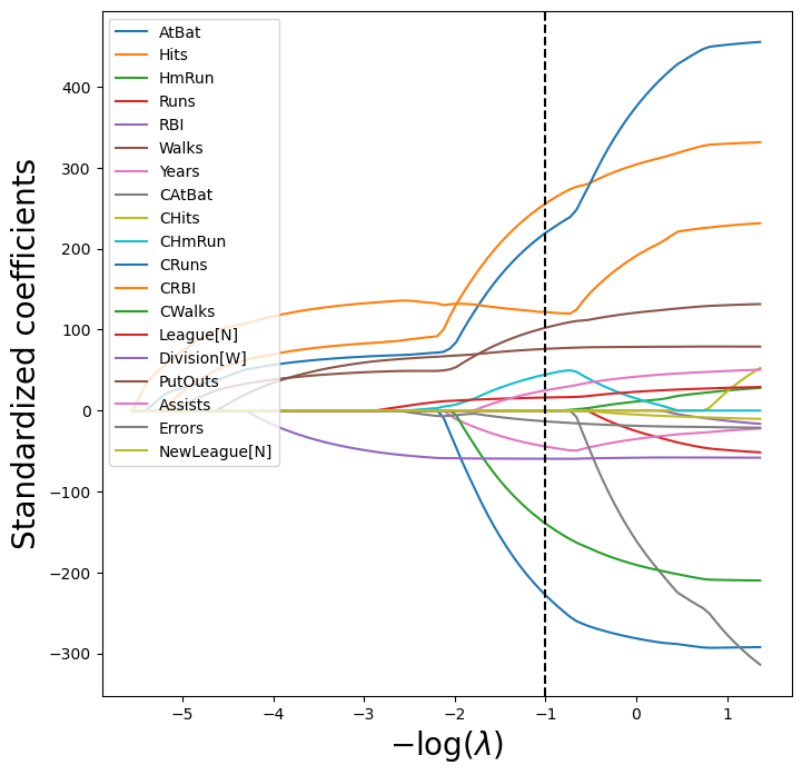

lassoCV_fig, ax = subplots(figsize=(8,8))
ax.errorbar(-np.log(tuned_lasso.alphas_),
            tuned_lasso.mse_path_.mean(1),
            yerr=tuned_lasso.mse_path_.std(1) / np.sqrt(K))
ax.axvline(-np.log(tuned_lasso.alpha_), c='k', ls='--')
ax.set_ylim([50000,250000])
ax.set_xlabel('$-\\log(\\lambda)$', fontsize=20)
ax.set_ylabel('Cross-validated MSE', fontsize=20);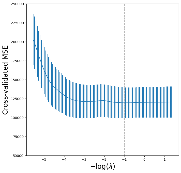

We can compare to ridge regression:

lambdas = 10**np.linspace(8, -2, 100) / Y.std()

ridgeCV = skl.ElasticNetCV(alphas=lambdas, # need to provide for ridge
                           l1_ratio=0, # l1_ratio=0 for ridge!
                           cv=K)
pipeCV = Pipeline(steps=[('scaler', scaler),
                         ('ridge', ridgeCV)])
pipeCV.fit(X, Y)
tuned_ridge = pipeCV.named_steps['ridge']

tuned_ridge.coef_

array([-222.80877051,  238.77246614,    3.21103754,   -2.93050845,
          3.64888723,  108.90953869,  -50.81896152, -105.15731984,
        122.00714801,   57.1859509 ,  210.35170348,  118.05683748,
       -150.21959435,   30.36634231,  -61.62459095,   77.73832472,
         40.07350744,  -25.02151514,  -13.68429544])

We can see the coefficients are not exactly zero.

lambdas, soln_array = skl.ElasticNet.path(Xs, Y, l1_ratio=0, alphas=lambdas)[:2]
soln_path = pd.DataFrame(soln_array.T,columns=dat.columns, index=-np.log(lambdas))

path_fig, ax = subplots(figsize=(8,8))
soln_path.plot(ax=ax, legend=False)
ax.set_xlabel('$-\\log(\\lambda)$', fontsize=20)
ax.set_ylabel('Standardized coefficiients', fontsize=20);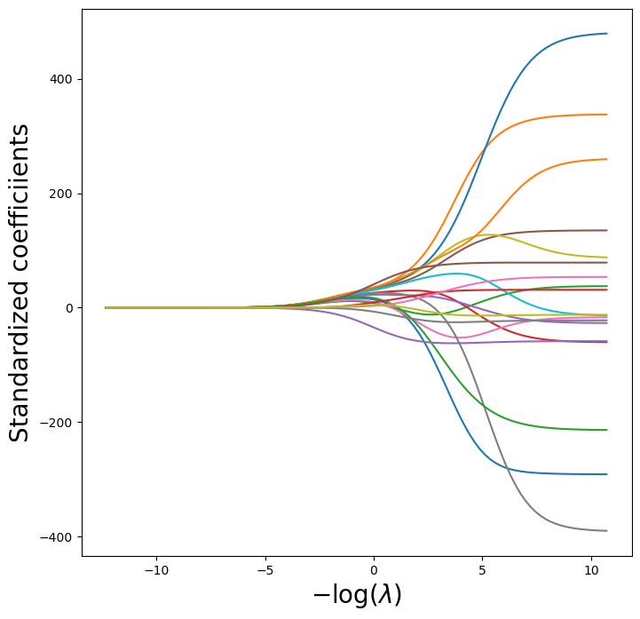

tuned_ridge = pipeCV.named_steps['ridge']
ridgeCV_fig, ax = subplots(figsize=(8,8))
ax.errorbar(-np.log(lambdas),
            tuned_ridge.mse_path_.mean(1),
            yerr=tuned_ridge.mse_path_.std(1) / np.sqrt(K))
ax.axvline(-np.log(tuned_ridge.alpha_), c='k', ls='--')
ax.set_xlabel('$-\\log(\\lambda)$', fontsize=20)
ax.set_ylabel('Cross-validated MSE', fontsize=20);