Lecture 4 - Classification

import numpy as np
import matplotlib.pyplot as plt

import warnings
warnings.filterwarnings('ignore')

Logistic Regression

Data Example

np.random.seed(2)

def sigmoid(z):
    # equivalent to e^(z)/(1 + e^{-z})
    return 1 / (1 + np.exp(-z))

n = 50

# Generate a synthetic dataset with a single feature
X = np.random.randn(n, 1) 

beta1 = 1
beta0 = -1

Y = np.random.binomial(1, sigmoid(beta0 + beta1 * X))
Y = Y.ravel()


## plot X against Y
plt.scatter(X, Y)
plt.xlabel('X')
plt.ylabel('Y')
plt.show()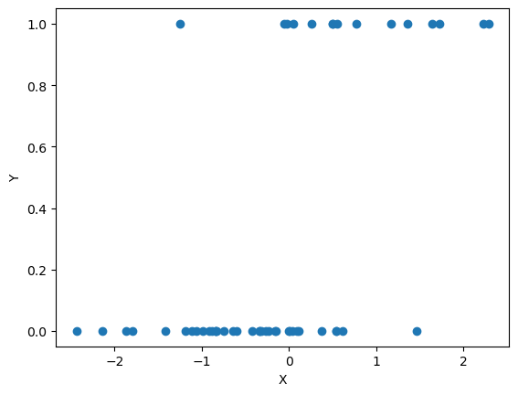

Gradient descent demonstration

def compute_loss(X, y, weights):
    n = X.shape[0]
    prob_pred = sigmoid(X @ weights)
    loss = (-1 / n) * np.sum(y * np.log(prob_pred) + (1 - y) * np.log(1 - prob_pred))
    return loss


def gradient_descent(X, y, weights, learning_rate, iterations):
    n = X.shape[0]

    loss = compute_loss(X, y, weights)
    loss_history = [loss]
    weight_history = [weights.copy()]

    for i in range(iterations):
        prob_pred = sigmoid(X @ weights)
        gradient = X.T @ (prob_pred - y) / n    
        weights -= learning_rate * gradient   ## weights = weights - learning_rate * gradient
        loss = compute_loss(X, y, weights)
        loss_history.append(loss)
        weight_history.append(weights.copy())
    
    return weights, loss_history, weight_history

# Add intercept to X
Xint = np.hstack((np.ones((X.shape[0], 1)), X))

# Initialize weights
init_weights = np.array([3.0, -3.0])

# Perform Gradient Descent
learning_rate = 1
niter = 50
weights, loss_history, weight_history = gradient_descent(Xint, Y, init_weights, learning_rate, iterations=niter)

## compare estimated weights with true weights
print('Estimated weights:', weights)
print('True weights:', np.array([beta0, beta1]))

Estimated weights: [-1.002386    1.78334711]
True weights: [-1  1]

# Create a grid for contour plot
beta0_range = np.linspace(-5, 5, 100)
beta1_range = np.linspace(-5, 5, 100)
B0, B1 = np.meshgrid(beta0_range, beta1_range)

# Compute loss for each combination in the grid
Loss = np.zeros(B0.shape)
for i in range(B0.shape[0]):
    for j in range(B0.shape[1]):
        Loss[i, j] = compute_loss(Xint, Y, np.array([B0[i, j], B1[i, j]]))

# Plotting
plt.figure(figsize=(8, 6))
# Contour plot for the loss
contour = plt.contour(B0, B1, Loss, levels=np.logspace(-2, 2, 70), cmap='viridis')
plt.clabel(contour, inline=True, fontsize=8)

# Overlay the trajectory of beta
beta_trajectory = np.array(weight_history)
plt.plot(beta_trajectory[:, 0], beta_trajectory[:, 1], '-o', color='red', label='Trajectory of Beta', lw=1, markersize=2)

plt.title('Contour Plot of Loss with Trajectory of Beta')
plt.xlabel('Beta 0 (Intercept)')
plt.ylabel('Beta 1 (Feature Weight)')
plt.legend()
plt.show()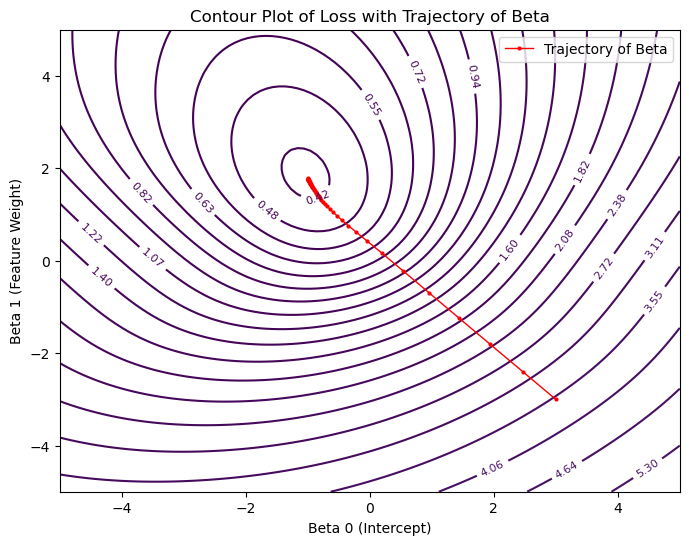

# Plot for Loss over Iterations
plt.plot(loss_history, '-o', markersize=2, lw=1)
plt.title('Loss over Iterations')
plt.xlabel('Iterations')
plt.ylabel('Loss')
plt.grid(True)

plt.tight_layout()
plt.show()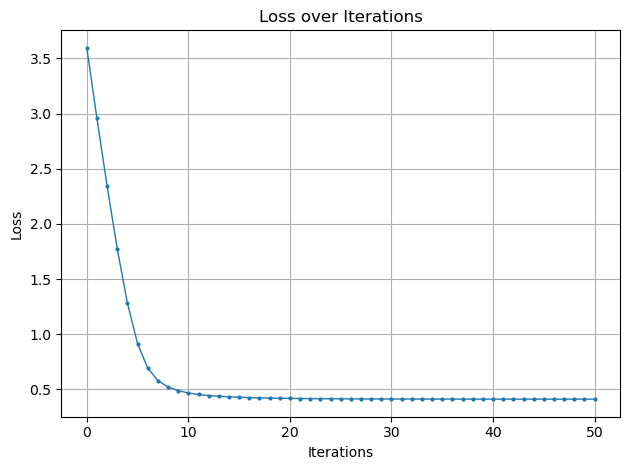

import matplotlib.pyplot as plt

# Scatter plot of X vs Y
plt.scatter(X, Y, alpha=0.5)
plt.xlabel('X')
plt.ylabel('Y')

# Generate x values for the sigmoid curve
x_vals = np.linspace(X.min(), X.max(), 100)
# Compute sigmoid with learned weights
sigmoid_vals = sigmoid(weights[0] + weights[1] * x_vals)
plt.plot(x_vals, sigmoid_vals, color='red', label='Fitted Model')
plt.legend()
plt.show()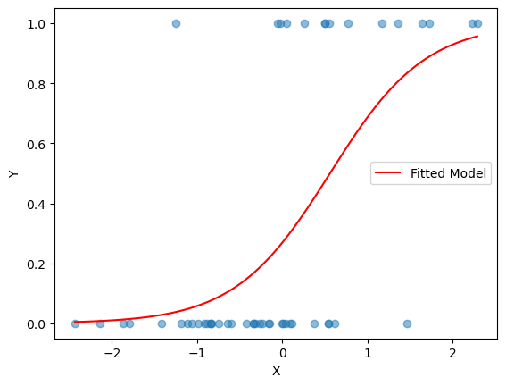

Stock Market Data

Adapted from Introduction to Statistical Learning with Python (link)

We now examine the Smarket data, which is part of the ISLP library. This data set consists of percentage returns for the S&P 500 stock index over 1,250 days, from the beginning of 2001 until the end of 2005. For each date, we have recorded the percentage returns for each of the five previous trading days, Lag1 through Lag5. We have also recorded Volume (the number of shares traded on the previous day, in billions), Today (the percentage return on the date in question) and Direction (whether the market was Up or Down on this date).

If you do not have the ISLP package, install it by going to your terminal (e.g. in VSCode or Anaconda Prompt):

conda activate stat486
pip install ISLP

import numpy as np
import pandas as pd
import statsmodels.api as sm
from ISLP import load_data
from ISLP import confusion_table

Loading the SMarket data:

Smarket = load_data('Smarket')
Smarket

	Year	Lag1	Lag2	Lag3	Lag4	Lag5	Volume	Today	Direction
0	2001	0.381	-0.192	-2.624	-1.055	5.010	1.19130	0.959	Up
1	2001	0.959	0.381	-0.192	-2.624	-1.055	1.29650	1.032	Up
2	2001	1.032	0.959	0.381	-0.192	-2.624	1.41120	-0.623	Down
3	2001	-0.623	1.032	0.959	0.381	-0.192	1.27600	0.614	Up
4	2001	0.614	-0.623	1.032	0.959	0.381	1.20570	0.213	Up
...	...	...	...	...	...	...	...	...	...
1245	2005	0.422	0.252	-0.024	-0.584	-0.285	1.88850	0.043	Up
1246	2005	0.043	0.422	0.252	-0.024	-0.584	1.28581	-0.955	Down
1247	2005	-0.955	0.043	0.422	0.252	-0.024	1.54047	0.130	Up
1248	2005	0.130	-0.955	0.043	0.422	0.252	1.42236	-0.298	Down
1249	2005	-0.298	0.130	-0.955	0.043	0.422	1.38254	-0.489	Down

1250 rows × 9 columns

Smarket.columns

Index(['Year', 'Lag1', 'Lag2', 'Lag3', 'Lag4', 'Lag5', 'Volume', 'Today',
       'Direction'],
      dtype='object')

We compute the correlation matrix using the corr() method for data frames, which produces a matrix that contains all of the pairwise correlations among the variables.

By instructing pandas to use only numeric variables, the corr() method does not report a correlation for the Direction variable because it is qualitative.

Smarket.corr(numeric_only=True)

	Year	Lag1	Lag2	Lag3	Lag4	Lag5	Volume	Today
Year	1.000000	0.029700	0.030596	0.033195	0.035689	0.029788	0.539006	0.030095
Lag1	0.029700	1.000000	-0.026294	-0.010803	-0.002986	-0.005675	0.040910	-0.026155
Lag2	0.030596	-0.026294	1.000000	-0.025897	-0.010854	-0.003558	-0.043383	-0.010250
Lag3	0.033195	-0.010803	-0.025897	1.000000	-0.024051	-0.018808	-0.041824	-0.002448
Lag4	0.035689	-0.002986	-0.010854	-0.024051	1.000000	-0.027084	-0.048414	-0.006900
Lag5	0.029788	-0.005675	-0.003558	-0.018808	-0.027084	1.000000	-0.022002	-0.034860
Volume	0.539006	0.040910	-0.043383	-0.041824	-0.048414	-0.022002	1.000000	0.014592
Today	0.030095	-0.026155	-0.010250	-0.002448	-0.006900	-0.034860	0.014592	1.000000

Smarket.plot(y='Volume');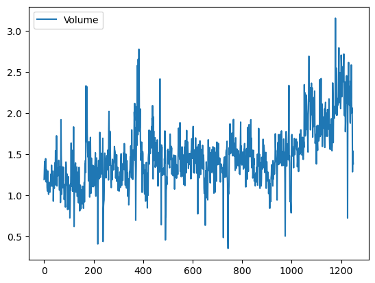

allvars = Smarket.columns.drop(['Today', 'Direction', 'Year'])
X = Smarket[allvars]
Xint = np.hstack((np.ones((X.shape[0], 1)), X))
y = Smarket.Direction == 'Up'

train = (Smarket.Year < 2005)
X_train, X_test = Xint[train], Xint[~train]
y_train, y_test = y[train], y[~train]

Logistic Regression

Next, we will fit a logistic regression model in order to predict Direction using Lag1 through Lag5 and Volume. The sm.GLM() function fits generalized linear models, a class of models that includes logistic regression. Alternatively, the function sm.Logit() fits a logistic regression model directly. The syntax of sm.GLM() is similar to that of sm.OLS(), except that we must pass in the argument family=sm.families.Binomial() in order to tell statsmodels to run a logistic regression rather than some other type of generalized linear model.

glm = sm.GLM(y_train,
             X_train,
             family=sm.families.Binomial())
results = glm.fit()
coeffs = results.params

features_list = ['Intercept'] + list(X.columns)
print("Coefficients:")
for i, f in enumerate(features_list):
    print(f"{f}: {coeffs[i]:.4f}")

Coefficients:
Intercept: 0.1912
Lag1: -0.0542
Lag2: -0.0458
Lag3: 0.0072
Lag4: 0.0064
Lag5: -0.0042
Volume: -0.1163

probs = results.predict(X_test)

# turn predictions in to labels
labels = np.array(['Down']*len(probs))
labels[probs>0.5] = "Up"

# turn test data into labels
L_test = np.array(['Down']*len(probs))
L_test[y_test == 1] = 'Up'

confusion_table(labels, L_test)

Truth	Down	Up
Predicted
Down	77	97
Up	34	44

np.mean(labels == L_test), (77+44)/len(L_test)

(np.float64(0.4801587301587302), 0.4801587301587302)

It is worse than random guessing!

Let’s try just Lag 1 and Lag 2.

X = Smarket[['Lag1', 'Lag2']]
Xint = np.hstack((np.ones((X.shape[0], 1)), X))
y = Smarket.Direction == 'Up'

train = (Smarket.Year < 2005)
X_train, X_test = Xint[train], Xint[~train]
y_train, y_test = y[train], y[~train]

glm_train = sm.GLM(y_train,
                   X_train,
                   family=sm.families.Binomial())
results = glm_train.fit()
probs = results.predict(exog=X_test)

labels = np.array(['Down']*len(y_test))
labels[probs>0.5] = 'Up'

L_test = np.array(['Down']*len(probs))
L_test[y_test == 1] = 'Up'

confusion_table(labels, L_test)

Truth	Down	Up
Predicted
Down	35	35
Up	76	106

np.mean(labels == L_test)

np.float64(0.5595238095238095)

A bit better! We will talk about how to do more systematic feature selection next class.