Lecture 2b - Supervised Learning

import pandas as pd
import numpy as np
import matplotlib.pyplot as plt
from sklearn.preprocessing import StandardScaler

np.random.seed(1)

import warnings
warnings.filterwarnings('ignore')

Data

We consider the Kings County housing dataset. It includes homes sold between May 2014 and May 2015.

Specifically, we focuse on the Rainier Valley zipcode.

# Load the dataset
house = pd.read_csv("data/rainier_valley_house.csv")

Here are the features:

house.columns

Index(['Unnamed: 0', 'id', 'date', 'price', 'bedrooms', 'bathrooms',
       'sqft_living', 'sqft_lot', 'floors', 'waterfront', 'view', 'condition',
       'grade', 'sqft_above', 'sqft_basement', 'yr_built', 'yr_renovated',
       'zipcode', 'lat', 'long', 'sqft_living15', 'sqft_lot15'],
      dtype='object')

# number of houses
print(f"number of houses:  {house.shape[0]}")

plt.boxplot(house['price'])
plt.title('Price Boxplot')
# make plot small in jupyter output
plt.gcf().set_size_inches(4, 3)

plt.show()

number of houses:  508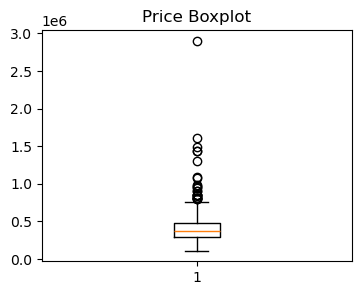

## For houses with 0, 1, 2, ... bedrooms, show their median price
print(house.groupby('bedrooms')['price'].median().reset_index())

   bedrooms     price
0         0  228000.0
1         1  299000.0
2         2  325000.0
3         3  365000.0
4         4  447500.0
5         5  425000.0
6         6  462500.0
7         7  370500.0

# Filtering houses priced under 1 million
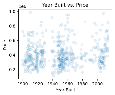
house = house[house['price'] < 1e6]

## Plot year built vs. price
plt.scatter(house['yr_built'], house['price'], alpha=0.1)
plt.xlabel('Year Built')
plt.ylabel('Price')
plt.title('Year Built vs. Price')
plt.gcf().set_size_inches(4, 3)
plt.show()

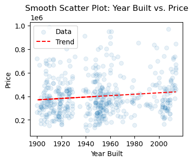
## Smooth scatter plot of year built vs. price
plt.scatter(house['yr_built'], house['price'], alpha=0.1, label='Data')
z = np.polyfit(house['yr_built'], house['price'], 1)
p = np.poly1d(z)
plt.plot(house['yr_built'], p(house['yr_built']), "r--", label='Trend')
plt.xlabel('Year Built')
plt.ylabel('Price')
plt.title('Smooth Scatter Plot: Year Built vs. Price')
plt.legend()
plt.gcf().set_size_inches(4, 3)
plt.show()

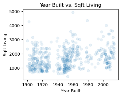
## Plot year built vs. sqft_living
plt.scatter(house['yr_built'], house['sqft_living'], alpha=0.1)
plt.xlabel('Year Built')
plt.ylabel('Sqft Living')
plt.title('Year Built vs. Sqft Living')
plt.gcf().set_size_inches(4, 3)
plt.show()


## Pairwise plot of price, bedrooms, and sqft_living
#pd.plotting.scatter_matrix(house[['price', 'bedrooms', 'sqft_living']], alpha=0.1, figsize=(10, 10))
#plt.show()

## Group by condition and calculate mean price
print(house.groupby('condition')['price'].mean().reset_index())

   condition          price
0          1  227000.000000
1          2  246749.705882
2          3  396841.120482
3          4  420201.384615
4          5  433258.152174

plt.figure(figsize=(10, 8))
sc = plt.scatter(house['long'], house['lat'], c=house['price'], cmap='viridis', alpha=0.5)
plt.colorbar(sc, label='Price ($)')
plt.xlabel('Longitude')
plt.ylabel('Latitude')
plt.title('House Location and Price')
plt.gcf().set_size_inches(5, 4)
plt.show()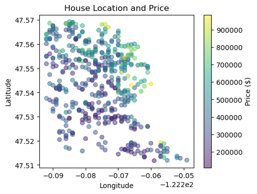

K-Nearest Neighbors

# We will consider this subset of features
features = ["floors", "grade", "condition", "view", "sqft_living",
            "sqft_lot", "sqft_basement", "yr_built", "yr_renovated",
            "bedrooms", "bathrooms", "lat", "long"]

Y = house['price'] / 1000
X = house[features]

## Standardize the features
scaler = StandardScaler()
X_stan = scaler.fit_transform(X)

## Split the data into training and test sets
n_train = 400
n_test = 100

idx = np.random.permutation(len(Y))
X_stan = X_stan[idx]
Y = Y.iloc[idx]

X_train = X_stan[:n_train]
X_test = X_stan[n_train:(n_train + n_test)]
Y_train = Y[:n_train]
Y_test = Y[n_train:n_train + n_test]

## Implement KNN
K = 7
Y_pred = []

for test_point in X_test:
    distances = np.sqrt(((X_train - test_point)**2).sum(axis=1))
    nearest_neighbors_indices = distances.argsort()[:K]
    Y_pred.append(Y_train.iloc[nearest_neighbors_indices].mean())

Y_pred = np.array(Y_pred)
Y_pred_baseline = Y_train.mean()

# Evaluate test error
test_error = np.sqrt(((Y_test - Y_pred) ** 2).mean())
baseline_error = np.sqrt(((Y_test - Y_pred_baseline) ** 2).mean())
print(f"Test RMSE of KNN: {test_error:.3f}   Baseline RMSE: {baseline_error:.3f}")

#print test R-squared
R2 = 1 - test_error**2 / baseline_error**2
print(f"Test R-squared of KNN: {R2:.3f}")

Test RMSE of KNN: 130.075   Baseline RMSE: 186.689
Test R-squared of KNN: 0.515

from sklearn.model_selection import train_test_split
from sklearn.neighbors import KNeighborsRegressor

# Split the data into training and test sets
X_train, X_test, Y_train, Y_test = train_test_split(X_stan, Y, test_size=100, train_size=400, random_state=1)

train_errs = []
test_errs = []

for K in range(1, 30):
    knn = KNeighborsRegressor(n_neighbors=K)
    knn.fit(X_train, Y_train)
    Y_train_pred = knn.predict(X_train)
    Y_pred = knn.predict(X_test)

    # Evaluate test error
    train_error = np.sqrt((Y_train - Y_train_pred) ** 2).mean()
    test_error = np.sqrt(((Y_test - Y_pred) ** 2).mean())
    
    train_errs.append(train_error)
    test_errs.append(test_error)

plt.plot(range(1, 30), train_errs, marker='o', label='train error')
plt.plot(range(1, 30), test_errs, marker='o', label='test error')
plt.legend()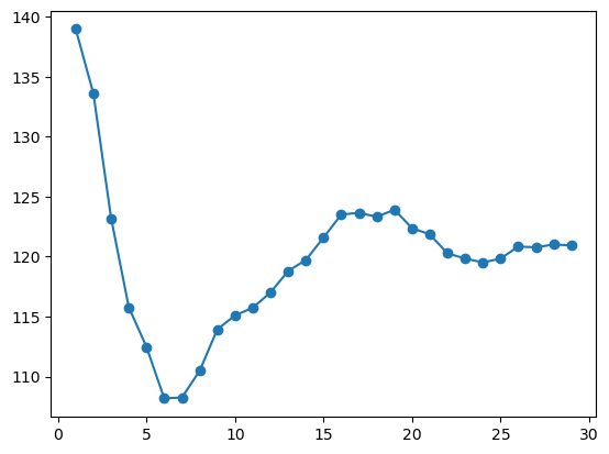

The test error is minimized at K=3.