Caveat for Conformal Inference

This simulation shows that we only get (1-\alpha)-coverage ON AVERAGE over the calibration set. That is, if we fix the calibration set, our coverage is not guaranteed.

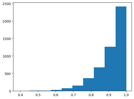
Below, we see the distribution of coverages for a fixed calibration set of size 10.

import numpy as np
import matplotlib.pyplot as plt
from scipy.stats import beta

# Parameters
N = 10  # Total number of variables
nprob = 1000  # samples to estimate coverage probability
ndraw = 5000 # estimating beta distribution

alpha = 0.1

preds10 = np.zeros((ndraw, nprob))

for i in range(ndraw):

    preds = []
    # fixed calibration set
    observed_variables = np.random.normal(0, 1, N)
    # quantile of fixed calibration set
    qhat = np.quantile(observed_variables, np.ceil((1-alpha) * (N+1)) / N)

    for j in range(nprob):

        # Generate the N-th random variable
        new_variable = np.random.normal(0, 1, 1)
        # is this variable in the prediction set???
        preds10[i, j] = (new_variable < qhat)

/var/folders/f0/m7l23y8s7p3_0x04b3td9nyjr2hyc8/T/ipykernel_4161/1945614140.py:27: DeprecationWarning: Conversion of an array with ndim > 0 to a scalar is deprecated, and will error in future. Ensure you extract a single element from your array before performing this operation. (Deprecated NumPy 1.25.)
  preds10[i, j] = (new_variable < qhat)

# each row corresponds to a fixed calibration set
plt.hist(preds10.mean(1))

(array([2.000e+00, 7.000e+00, 1.200e+01, 3.000e+01, 7.800e+01, 1.520e+02,
        3.680e+02, 6.730e+02, 1.265e+03, 2.413e+03]),
 array([0.39 , 0.451, 0.512, 0.573, 0.634, 0.695, 0.756, 0.817, 0.878,
        0.939, 1.   ]),
 <BarContainer object of 10 artists>)

If you average over the calibration sets, we recover (1-\alpha) coverage.

preds10.mean()

0.9108314

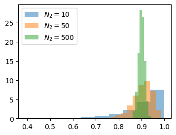
If we increase the size of our calibration set, the coverage probabilities are closer to (1-\alpha) (for a fixed calibration set.)

# Parameters
N = 50  # Total number of variables
nprob = 1000  # Number of simulations
ndraw = 5000

alpha = 0.1

preds50 = np.zeros((ndraw, nprob))

for i in range(ndraw):

    preds = []

    observed_variables = np.random.normal(0, 1, N)

    qhat = np.quantile(observed_variables, np.ceil((1-alpha) * (N+1)) / N)

    for j in range(nprob):

        # Generate the N-th random variable
        new_variable = np.random.normal(0, 1, 1)

        preds50[i, j] = (new_variable < qhat)

/var/folders/f0/m7l23y8s7p3_0x04b3td9nyjr2hyc8/T/ipykernel_4161/3492330592.py:23: DeprecationWarning: Conversion of an array with ndim > 0 to a scalar is deprecated, and will error in future. Ensure you extract a single element from your array before performing this operation. (Deprecated NumPy 1.25.)
  preds50[i, j] = (new_variable < qhat)

# each row corresponds to a fixed calibration set
plt.hist(preds50.mean(1))

# Parameters
N = 1000  # Total number of variables
nprob = 1000  # Number of simulations
ndraw = 5000

alpha = 0.1

preds1000 = np.zeros((ndraw, nprob))

for i in range(ndraw):

    preds = []

    observed_variables = np.random.normal(0, 1, N)

    qhat = np.quantile(observed_variables, np.ceil((1-alpha) * (N+1)) / N)

    for j in range(nprob):

        # Generate the N-th random variable
        new_variable = np.random.normal(0, 1, 1)

        preds1000[i, j] = (new_variable < qhat)

/var/folders/f0/m7l23y8s7p3_0x04b3td9nyjr2hyc8/T/ipykernel_4161/2919383409.py:23: DeprecationWarning: Conversion of an array with ndim > 0 to a scalar is deprecated, and will error in future. Ensure you extract a single element from your array before performing this operation. (Deprecated NumPy 1.25.)
  preds1000[i, j] = (new_variable < qhat)

plt.figure(figsize=(4,3))
plt.hist(preds10.mean(axis=1),density=True,alpha=0.5, label=r'$N_2=10$')
plt.hist(preds50.mean(axis=1),density=True,alpha=0.5, label=r'$N_2=50$')
plt.hist(preds1000.mean(axis=1),density=True,alpha=0.5, label=r'$N_2=500$')
plt.legend()

print(preds10.mean())
print(preds50.mean())
print(preds1000.mean())

0.9061804
0.9037104
0.902485

Why does this happen? With a smaller, fixed calibration set, we get worse approximations to the distribution, and the ranks are not uniform!!!

# Parameters
N = 10  
ndraw = 5000

rank = np.zeros((ndraw))
observed_variables = np.random.normal(0, 1, N-1)

for i in range(ndraw):
    
    new_variable = np.random.normal(0, 1, 1)

    variables = np.concatenate([observed_variables,new_variable])
    variables_rank = variables.argsort().argsort() + 1
    rank[i] = variables_rank[-1]

plt.hist(rank)

(array([ 365.,  420.,  167.,   50., 1575.,  141.,  969.,  270.,  357.,
         686.]),
 array([ 1. ,  1.9,  2.8,  3.7,  4.6,  5.5,  6.4,  7.3,  8.2,  9.1, 10. ]),
 <BarContainer object of 10 artists>)

In contrast, the ranks are uniform when we re-draw the calibration set for each new variable (i.e. average over calibration set).

# Parameters
N = 10  
ndraw = 5000

rank = np.zeros((ndraw))

for i in range(ndraw):
    
    observed_variables = np.random.normal(0, 1, N-1)
    new_variable = np.random.normal(0, 1, 1)

    variables = np.concatenate([observed_variables,new_variable])
    variables_rank = variables.argsort().argsort() + 1
    rank[i] = variables_rank[-1]

plt.hist(rank)

(array([499., 481., 515., 521., 497., 502., 524., 454., 512., 495.]),
 array([ 1. ,  1.9,  2.8,  3.7,  4.6,  5.5,  6.4,  7.3,  8.2,  9.1, 10. ]),
 <BarContainer object of 10 artists>)